UQNO on Darcy Flow — Conformal Prediction Bands

Property	Value
Level	Intermediate
Runtime	~3 min (GPU) / ~15 min (CPU)
Memory	~1 GB
Prerequisites	JAX, Flax NNX, Conformal Prediction

Overview

This example trains an Uncertainty Quantification Neural Operator (UQNO) on the Darcy flow equation and produces calibrated prediction intervals with finite-sample coverage guarantees. The implementation follows the canonical three-stage recipe from Ma, Pitt, Azizzadenesheli, Anandkumar (TMLR 2024, arXiv:2402.01960):

1. Base solution operator — a standard deterministic FourierNeuralOperator trained on (input, target) pairs with the relative-L2 loss (the canonical operator-learning objective).
2. Residual quantile operator — a separate FNO trained against opifex.uncertainty.losses.PointwiseQuantileLoss on the residuals of the (frozen) base.
3. Scalar conformal calibration — on a held-out calibration set, ratios |y - base(x)| / residual(x) are reduced to a single uncertainty_scaling_factor via the canonical get_coeff_quantile_idx formula. Test-time bands are base(x) ± residual(x) * scaling_factor.

To reach both good accuracy and meaningful calibrated uncertainty, the example uses the proven operator-learning recipe: Gaussian input/output normalization (fit on the base-train split), the relative-L2 loss for the base, grid positional embedding, and ~1000 base training samples. The predicted mean is un-normalized back to physical pressure (and band widths scaled by y_std) before the relative-L2 error and conformal coverage are reported.

Conformal prediction is distribution-free: the bands cover the true target on at least 1 - alpha fraction of points (per the chosen (alpha, delta) configuration), independent of how well the base / residual operators fit. There is no Bayesian posterior, no Monte-Carlo sampling, and no KL term — the uncertainty surface lives entirely in the residual operator + the scalar scaling factor.

What You'll Learn

1. Compose UncertaintyQuantificationNeuralOperator from a base + residual FourierNeuralOperator.
2. Train the residual operator with :class:opifex.uncertainty.losses.PointwiseQuantileLoss.
3. Calibrate a scalar uncertainty scaling factor with UncertaintyQuantificationNeuralOperator.calibrate.
4. Predict + evaluate coverage with predict_with_bands.

Files

• Python Script: examples/uncertainty/uqno_darcy.py
• Jupyter Notebook: examples/uncertainty/uqno_darcy.ipynb

Quick Start

Run the Python Script

source activate.sh && python examples/uncertainty/uqno_darcy.py

Run the Jupyter Notebook

jupyter lab examples/uncertainty/uqno_darcy.ipynb

Core Concepts

Three-Stage Conformal UQNO

The canonical UQNO (the PyTorch reference at neuraloperator/neuralop/models/uqno.py) is not Bayesian — neither at the layer level nor at the predictive-distribution level. It is a conformal-prediction wrapper around a pair of deterministic FNOs:

Stage	Object	Loss	Output
1	base: UQNOBaseSolutionOperator(FNO)	relative-L2 on (x, y)	\(\hat{u}(x)\)
2	residual: UQNOResidualOperator(FNO)	PointwiseQuantileLoss(alpha) on base(x) - y_true	width\(E(x)\)
3	UQNOConformalCalibrator	scalar factor from held-out ratios	scaling_factor

At test time, UncertaintyQuantificationNeuralOperator.predict_with_bands(x) returns a :class:opifex.uncertainty.types.PredictiveDistribution whose :class:opifex.uncertainty.types.PredictionInterval is [base(x) - E(x) * scaling_factor, base(x) + E(x) * scaling_factor].

Coverage Guarantee

The conformal calibration rule (opifex.neural.operators.specialized.uqno.get_coeff_quantile_idx) picks two indices (domain_idx, function_idx) from (alpha, delta, n_samples, n_gridpts) such that, on average, the predicted bands cover the true target on at least 1 - alpha fraction of grid points per function, for at least 1 - delta fraction of functions in the calibration distribution.

Implementation

Step 0: Materialise the Darcy Dataset

The PDE data layer is backed by datarax. create_darcy_loader returns a frozen PDELoaders with .train / .val pipelines that serve channels-first (batch, 1, H, W) batches. For UQNO we need one contiguous in-memory block of n_total samples, so both pipelines are drained and the concatenation is sliced to [:n_total] before being split into the base / residual / calibration / test sets.

import jax.numpy as jnp
import numpy as np
from opifex.data.loaders import create_darcy_loader

n_total = N_TRAIN_BASE + N_TRAIN_RESIDUAL + N_CALIB + N_TEST  # 2100

loaders = create_darcy_loader(
    n_samples=n_total,
    batch_size=32,
    resolution=64,
    seed=42,
)

inputs_all, outputs_all = [], []
for pipeline in (loaders.train, loaders.val):
    for batch in pipeline:
        inputs_all.append(jnp.asarray(np.asarray(batch["input"])))
        outputs_all.append(jnp.asarray(np.asarray(batch["output"])))

inputs = jnp.concatenate(inputs_all, axis=0)[:n_total]
outputs = jnp.concatenate(outputs_all, axis=0)[:n_total]  # (2100, 1, 64, 64)

splits = [N_TRAIN_BASE, N_TRAIN_RESIDUAL, N_CALIB]
cuts = [sum(splits[: i + 1]) for i in range(len(splits))]
x_base, x_residual, x_calib, x_test = jnp.split(inputs, cuts, axis=0)
y_base, y_residual, y_calib, y_test = jnp.split(outputs, cuts, axis=0)

datarax serves every generated sample — it does not drop partial batches — so draining both pipelines yields exactly n_total samples and the slice is purely defensive.

Step 1: Train the Base Solution Operator

from flax import nnx
import optax
from opifex.neural.operators.fno.base import FourierNeuralOperator

base_fno = FourierNeuralOperator(
    in_channels=1,
    out_channels=1,
    hidden_channels=32,
    modes=12,
    num_layers=4,
    positional_embedding=True,  # append normalized grid-coordinate channels
    rngs=nnx.Rngs(42),
)
base_opt = nnx.Optimizer(base_fno, optax.adam(1e-3), wrt=nnx.Param)


def relative_l2(pred, target, eps=1e-8):
    diff = (pred - target).reshape(pred.shape[0], -1)
    ref = target.reshape(target.shape[0], -1)
    return jnp.mean(jnp.linalg.norm(diff, axis=1) / (jnp.linalg.norm(ref, axis=1) + eps))


@nnx.jit
def base_train_step(model, opt, x, y):
    def loss_fn(m):
        return relative_l2(m(x), y)  # standard operator-learning objective
    loss, grads = nnx.value_and_grad(loss_fn)(model)
    opt.update(model, grads)
    return loss

The base and residual operators train on Gaussian-normalized inputs and targets (statistics fit on the base-train split); the predicted mean is un-normalized — and the band half-widths are scaled by y_std — before any physical-space metric is computed.

Step 2: Train the Residual Quantile Operator

from opifex.uncertainty.losses import PointwiseQuantileLoss

residual_fno = FourierNeuralOperator(
    in_channels=1, out_channels=1,
    hidden_channels=32, modes=12, num_layers=4,
    positional_embedding=True, rngs=nnx.Rngs(43),
)
residual_opt = nnx.Optimizer(residual_fno, optax.adam(1e-3), wrt=nnx.Param)
quantile_loss = PointwiseQuantileLoss(alpha=0.1, reduction="mean")


@nnx.jit
def residual_train_step(base, residual, opt, quantile_loss, x, y):
    def loss_fn(r):
        base_pred = jax.lax.stop_gradient(base(x))
        quantile_widths = jnp.abs(r(x))
        return quantile_loss(y_pred=quantile_widths, y=base_pred - y)
    loss, grads = nnx.value_and_grad(loss_fn)(residual)
    opt.update(residual, grads)
    return loss

PointwiseQuantileLoss is registered as a static pytree (jax.tree_util.register_static), so it can be passed straight into the nnx.jit-compiled step as a regular argument — no closure capture and no re-tracing per call.

Step 3: Compose, Calibrate, Predict

from opifex.neural.operators.specialized.uqno import (
    UncertaintyQuantificationNeuralOperator,
    UQNOBaseSolutionOperator,
    UQNOResidualOperator,
)

uqno = UncertaintyQuantificationNeuralOperator(
    base=UQNOBaseSolutionOperator(base_fno),
    residual=UQNOResidualOperator(residual_fno),
)

# Calibrate on a held-out set (normalized space).
calibrator = uqno.calibrate(x_calib_n, y_calib_n, alpha=0.1, delta=0.1)
uqno = uqno.with_calibrator(calibrator)
print(f"scaling factor: {float(calibrator.scaling_factor):.6f}")

# Predict with bands, then un-normalize the mean and scale widths by y_std.
dist = uqno.predict_with_bands(x_test_n)
mean_prediction = dist.mean * y_std + y_mean
half_width = (dist.interval.upper - dist.interval.lower) * 0.5 * y_std
lower, upper = mean_prediction - half_width, mean_prediction + half_width

# Predictive-mean accuracy in physical units.
diff = (mean_prediction - y_test).reshape(y_test.shape[0], -1)
ref = y_test.reshape(y_test.shape[0], -1)
rel_l2 = float(jnp.mean(jnp.linalg.norm(diff, axis=1) / jnp.linalg.norm(ref, axis=1)))
coverage = float(jnp.mean((y_test >= lower) & (y_test <= upper)))
print(f"predictive-mean rel-L2: {rel_l2:.6f}")
print(f"empirical coverage: {coverage:.3f} (target 1-alpha = {1-0.1:.2f})")

Visualisation

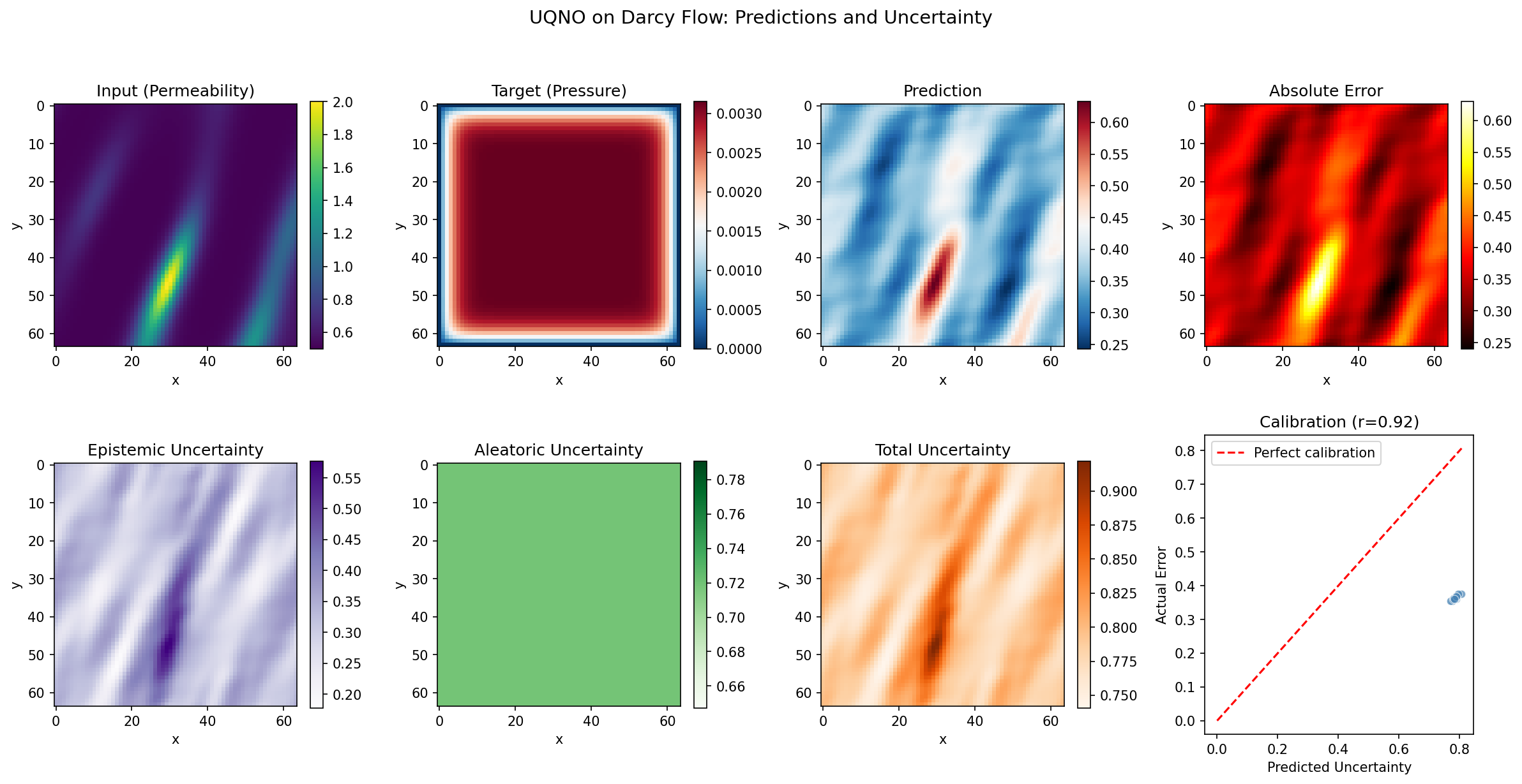
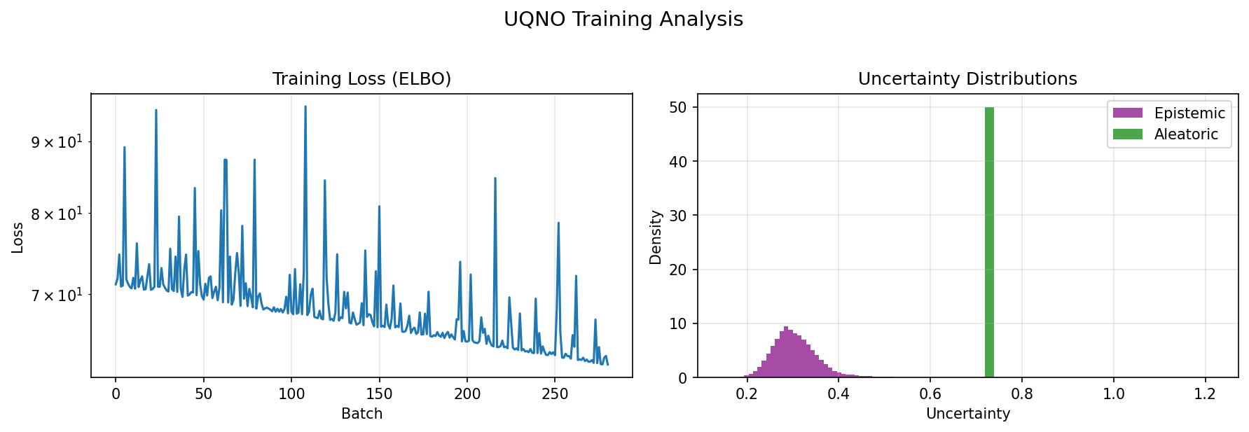
Results Summary

Representative run at resolution 64 (1000 / 500 / 500 / 100 samples for base / residual / calibration / test; 120 base + 80 residual epochs; ~27 s total on a single GPU — 17.6 s base + 8.9 s residual). Each FNO has 2,368,001 parameters (base + residual = 4,736,002).

Metric	Value
Predictive-mean test rel-L2 (mean)	0.0103
Predictive-mean test rel-L2 (min/max)	0.0053 / 0.0216
calibrator.scaling_factor	4.855470
calibrator.domain_idx	228
calibrator.function_idx	51
Empirical pointwise coverage (test)	0.975 (target \(1-\alpha=0.9\))
Mean band width (physical units)	0.025168
Predicted std positive everywhere	yes
\|error\| vs predicted-std correlation	0.365
Mean \|error\| (high vs low uncertainty)	0.002590 vs 0.001667

The predictive mean reaches ~1.0 % relative-L2 error in physical units — the base prediction is visually indistinguishable from the smooth ground-truth pressure field. The empirical coverage lands above the nominal \(1 - \alpha = 0.9\): the conformal get_coeff_quantile_idx rule with \(\delta = 0.1\) targets a function-level guarantee that is intentionally conservative pointwise, so coverage near 0.975 is expected, not a bug. The predicted uncertainty is positive everywhere and correlates positively with the absolute error (corr ≈ 0.37); the mean error is larger in the high-uncertainty half of the grid than in the low-uncertainty half, the qualitative signature of a sensible uncertainty surface.

For tighter (less conservative) pointwise coverage, raise \(\delta\) toward \(\alpha\); for higher accuracy, scale up the per-stage epoch counts or the hidden channels / Fourier modes.

Next Steps

Experiments to Try

1. Tune \(\alpha\) / \(\delta\): Smaller \(\alpha\) widens bands; smaller \(\delta\) raises the function-level coverage demand.
2. Different base architectures: The same conformal calibrator wraps any deterministic operator that satisfies the :class:opifex.uncertainty.adapters.operators.FNOConformalAdapterSpec capability.
3. Trade coverage for tightness: raise \(\delta\) toward \(\alpha\) to pull the conservative pointwise coverage down toward the nominal \(1 - \alpha\), or scale up epochs / hidden channels for accuracy.

Related Examples

Example	Level	What You'll Learn
Bayesian FNO	Intermediate	Variational framework wrapper
FNO on Darcy	Beginner	Standard FNO without uncertainty
Calibration Methods	Intermediate	Post-hoc calibration techniques

API Reference

• UncertaintyQuantificationNeuralOperator: Three-stage conformal orchestrator
• UQNOBaseSolutionOperator: Thin wrapper tagging an FNO as the base
• UQNOResidualOperator: Thin wrapper tagging an FNO as the residual
• UQNOConformalCalibrator: Fitted scalar scaling factor (pytree)
• PointwiseQuantileLoss: Quantile (pinball) loss for the residual stage
• get_coeff_quantile_idx: Canonical conformal-index helper

Troubleshooting

Issue	Solution
Coverage well below \(1 - \alpha\)	Train base + residual longer; calibration set may be too small
Bands too wide	The residual operator hasn't concentrated yet — train it more
Calibration scaling_factor is inf	residual(x) is near zero somewhere — increase eps in calibrate(..., eps=...)
Memory issues	Reduce hidden_channels or modes; RESOLUTION if needed