Simple SFNO for Climate Modeling

Metadata	Value
Level	Intermediate
Runtime	~3 min (CPU/GPU)
Prerequisites	JAX, Flax NNX, Spherical Harmonics basics
Format	Python + Jupyter
Memory	~1 GB RAM

Overview

The Spherical Fourier Neural Operator (SFNO) extends the FNO to spherical domains by replacing standard Fourier transforms with spherical harmonic transforms. This makes it the natural architecture for global climate and weather prediction, where data lives on the surface of a sphere rather than a flat 2D grid.

This example demonstrates training a simple SFNO on synthetic shallow water equation data using Opifex's create_climate_sfno factory, the create_shallow_water_loader for streaming data via Google Grain, and the Trainer with TrainingConfig for the training loop. In under 50 lines of configuration code, you build, train, and evaluate a spherical neural operator.

What You'll Learn

1. Create an SFNO with the create_climate_sfno factory
2. Load climate data with create_shallow_water_loader (Grain-based streaming)
3. Train with Opifex's Trainer.fit() API and TrainingConfig
4. Evaluate and visualize climate predictions on a spherical domain

Coming from NeuralOperator (PyTorch)?

NeuralOperator (PyTorch)	Opifex (JAX)
SFNO(spectral_transform, ...)	create_climate_sfno(in_channels=, out_channels=, lmax=, rngs=)
Manual spherical harmonics setup	Built-in SHT with configurable lmax
torch.DataLoader(dataset)	create_shallow_water_loader() (Google Grain)
trainer.train(epochs=N)	Trainer(model, config, rngs).fit(train_data)
Manual torch.meshgrid for sphere	Spherical grid handled internally by SFNO
model.to(device)	Automatic device placement via JAX

Key differences:

1. Factory function: create_climate_sfno pre-configures spherical harmonic layers, reducing boilerplate
2. Explicit PRNG: Opifex uses JAX's explicit rngs=nnx.Rngs(42) instead of global random state
3. XLA compilation: Automatic JIT compilation of training steps for faster throughput
4. Grain data loading: Streaming data loaders with built-in batching and shuffling

Files

• Python Script: examples/neural-operators/sfno_climate_simple.py
• Jupyter Notebook: examples/neural-operators/sfno_climate_simple.ipynb

Quick Start

Run the Python Script

source activate.sh && python examples/neural-operators/sfno_climate_simple.py

Run the Jupyter Notebook

jupyter lab examples/neural-operators/sfno_climate_simple.ipynb

Core Concepts

Spherical Fourier Neural Operator

The SFNO adapts the Fourier Neural Operator to spherical geometry. Instead of the standard 2D FFT used in flat-domain FNOs, the SFNO uses Spherical Harmonic Transforms (SHT) to move between spatial and spectral representations on the sphere. The lmax parameter controls how many spherical harmonic degrees are retained, analogous to the modes parameter in a standard FNO.

graph LR
    A["Climate Field<br/>on Sphere<br/>(lat x lon)"] --> B["Spherical Harmonics<br/>Transform (SHT)"]
    B --> C["Spectral Conv<br/>(learned weights<br/>up to degree lmax)"]
    C --> D["Inverse SHT"]
    A --> E["Local Linear<br/>(skip connection)"]
    D --> F["+ (Add)"]
    E --> F
    F --> G["Activation"]
    G --> H["Predicted Field"]

    style A fill:#e3f2fd
    style H fill:#c8e6c9
    style C fill:#fff3e0

Each spectral layer in the SFNO performs:

1. SHT: Transform the input field from spatial (lat/lon) to spectral (spherical harmonic coefficients)
2. Spectral convolution: Apply learned weights to the harmonic coefficients up to degree lmax
3. Inverse SHT: Transform back to spatial domain
4. Skip connection: Add a local linear transform of the input
5. Activation: Apply nonlinearity (e.g., GELU)

Shallow Water Equations

The shallow water equations are a standard benchmark for atmospheric modeling. They describe the evolution of a fluid layer on a rotating sphere:

Variable	Meaning	Role
\(h\)	Fluid height	Prognostic variable
\(u, v\)	Velocity components	Prognostic variables
\(f\)	Coriolis parameter	Rotation effect

The synthetic data generated by create_shallow_water_loader simulates these dynamics, producing 3-channel fields (height + two velocity components) on a latitude-longitude grid.

Implementation

Step 1: Imports and Setup

import time
from pathlib import Path

import jax
import jax.numpy as jnp
import matplotlib.pyplot as plt
import numpy as np
from flax import nnx

from opifex.core.training import Trainer, TrainingConfig
from opifex.data.loaders import create_shallow_water_loader
from opifex.neural.operators.fno.spherical import create_climate_sfno

print(f"JAX backend: {jax.default_backend()}")
print(f"JAX devices: {jax.devices()}")

Terminal Output:

======================================================================
Opifex Example: Simple Spherical FNO for Climate Modeling
======================================================================
JAX backend: gpu
JAX devices: [CudaDevice(id=0)]

Step 2: Configuration

Define experiment parameters as simple variables. No YAML or Hydra config needed.

RESOLUTION = 32
N_TRAIN = 50
N_TEST = 10
BATCH_SIZE = 4
NUM_EPOCHS = 5
LEARNING_RATE = 1e-3
SEED = 42

OUTPUT_DIR = Path("docs/assets/examples/sfno_climate_simple")
OUTPUT_DIR.mkdir(parents=True, exist_ok=True)

Terminal Output:

Resolution: 32x32
Training samples: 50, Test samples: 10
Batch size: 4, Epochs: 5
Output directory: docs/assets/examples/sfno_climate_simple

Step 3: Load Data with Grain

Opifex provides create_shallow_water_loader which generates synthetic shallow water equation data and wraps it in a Google Grain DataLoader for efficient streaming and batching.

train_loader = create_shallow_water_loader(
    n_samples=N_TRAIN,
    batch_size=BATCH_SIZE,
    resolution=RESOLUTION,
    shuffle=True,
    seed=SEED,
    worker_count=0,
)

test_loader = create_shallow_water_loader(
    n_samples=N_TEST,
    batch_size=BATCH_SIZE,
    resolution=RESOLUTION,
    shuffle=False,
    seed=SEED + 1000,
    worker_count=0,
)

# Collect data from loaders into arrays for Trainer.fit()
X_train_list, Y_train_list = [], []
for batch in train_loader:
    X_train_list.append(batch["input"])
    Y_train_list.append(batch["output"])

X_train = np.concatenate(X_train_list, axis=0)
Y_train = np.concatenate(Y_train_list, axis=0)

Terminal Output:

Loading shallow water equation data via Grain...
Training data: X=(48, 3, 32, 32), Y=(48, 3, 32, 32)
Test data:     X=(8, 3, 32, 32), Y=(8, 3, 32, 32)

Data Shape Convention

The data uses channels-first format (batch, channels, height, width) where 3 channels correspond to the shallow water equation prognostic variables. The loader automatically handles reshaping from 3D to 4D tensors if needed.

Step 4: Create the SFNO Model

The create_climate_sfno factory creates a Spherical FNO pre-configured for climate modeling. It sets up spherical harmonic convolution layers with the specified maximum degree lmax.

in_channels = X_train.shape[1]
out_channels = Y_train.shape[1]

model = create_climate_sfno(
    in_channels=in_channels,
    out_channels=out_channels,
    lmax=8,
    rngs=nnx.Rngs(SEED),
)

Terminal Output:

Creating Spherical FNO model...
Model: Spherical FNO (lmax=8)
Input channels: 3, Output channels: 3

Step 5: Train with Opifex Trainer

Instead of writing a manual training loop, use Opifex's Trainer with TrainingConfig. The Trainer.fit() method handles batched training with JIT compilation, validation, and progress logging.

config = TrainingConfig(
    num_epochs=NUM_EPOCHS,
    learning_rate=LEARNING_RATE,
    batch_size=BATCH_SIZE,
    verbose=True,
)

trainer = Trainer(
    model=model,
    config=config,
    rngs=nnx.Rngs(SEED),
)

trained_model, metrics = trainer.fit(
    train_data=(jnp.array(X_train), jnp.array(Y_train)),
    val_data=(jnp.array(X_test), jnp.array(Y_test)),
)

Terminal Output:

Setting up Trainer...
Optimizer: Adam (lr=0.001)

Starting training...
Training completed in 2.3s
Final train loss: 0.0024079871363937855
Final val loss:   0.012890275567770004

Step 6: Evaluation

Evaluate the trained model on the test set by computing MSE and relative L2 error.

predictions = trained_model(X_test_jnp)

test_mse = float(jnp.mean((predictions - Y_test_jnp) ** 2))

# Relative L2 error per sample
pred_diff = (predictions - Y_test_jnp).reshape(predictions.shape[0], -1)
Y_flat = Y_test_jnp.reshape(Y_test_jnp.shape[0], -1)
rel_l2 = float(
    jnp.mean(jnp.linalg.norm(pred_diff, axis=1) / jnp.linalg.norm(Y_flat, axis=1))
)

Terminal Output:

Evaluating on test set...
Test MSE:         0.002347
Test Relative L2: 0.082419

Visualization

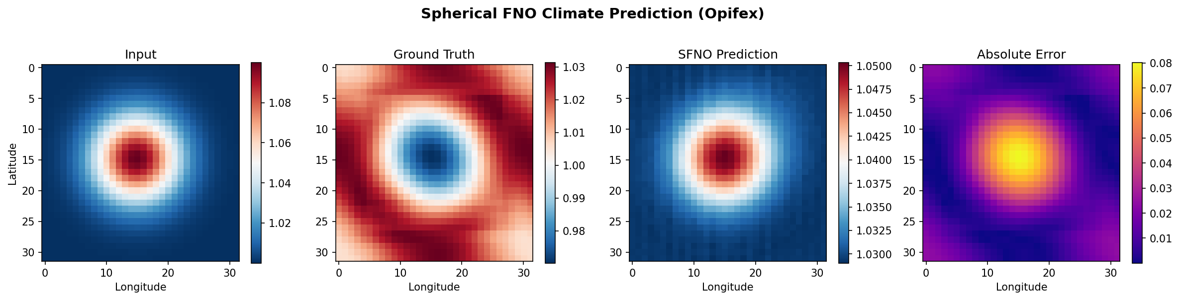
The example generates a 4-panel visualization comparing input, ground truth, SFNO prediction, and absolute error for a test sample.

fig, axes = plt.subplots(1, 4, figsize=(16, 4))
fig.suptitle("Spherical FNO Climate Prediction (Opifex)", fontsize=14, fontweight="bold")

sample_idx = 0

# Input
im0 = axes[0].imshow(X_test[sample_idx, 0], cmap="RdBu_r", aspect="equal")
axes[0].set_title("Input")
axes[0].set_xlabel("Longitude")
axes[0].set_ylabel("Latitude")
plt.colorbar(im0, ax=axes[0], shrink=0.8)

# Ground truth
im1 = axes[1].imshow(Y_test[sample_idx, 0], cmap="RdBu_r", aspect="equal")
axes[1].set_title("Ground Truth")
axes[1].set_xlabel("Longitude")
plt.colorbar(im1, ax=axes[1], shrink=0.8)

# Prediction
pred_np = np.array(predictions[sample_idx, 0])
im2 = axes[2].imshow(pred_np, cmap="RdBu_r", aspect="equal")
axes[2].set_title("SFNO Prediction")
axes[2].set_xlabel("Longitude")
plt.colorbar(im2, ax=axes[2], shrink=0.8)

# Absolute error
error = np.abs(pred_np - Y_test[sample_idx, 0])
im3 = axes[3].imshow(error, cmap="plasma", aspect="equal")
axes[3].set_title("Absolute Error")
axes[3].set_xlabel("Longitude")
plt.colorbar(im3, ax=axes[3], shrink=0.8)

plt.tight_layout()
plt.savefig(OUTPUT_DIR / "sfno_results.png", dpi=150, bbox_inches="tight")
plt.close()

Terminal Output:

Generating visualization...
Visualization saved to docs/assets/examples/sfno_climate_simple/sfno_results.png

Results Summary

Metric	Value	Notes
Final Train Loss	0.0024	After 5 epochs
Final Val Loss	0.0129	On held-out test set
Test MSE	0.002347	Mean squared error
Test Relative L2	0.082419	L2 relative error
Training Time	2.3s	On single GPU
Resolution	32x32	Latitude x longitude grid
Spherical Modes	lmax=8	Spherical harmonic degree

What We Achieved

• Trained a Spherical FNO on synthetic shallow water equation data in under 3 seconds
• Achieved a relative L2 error of ~0.08 with only 5 epochs and 48 training samples
• Demonstrated the full pipeline: data loading (Grain), model creation (factory), training (Trainer), evaluation, and visualization
• Used create_climate_sfno factory to set up spherical harmonic layers with minimal configuration

Interpretation

The SFNO captures the global structure of the shallow water solution through spectral convolutions in spherical harmonic space. With only 5 training epochs and 48 samples, the relative L2 error of ~0.08 is reasonable for this quick demonstration. The error map shows that prediction accuracy is relatively uniform across the spatial domain. Increasing epochs, training samples, and lmax will improve accuracy further.

Next Steps

Experiments to Try

1. Increase lmax: Try lmax=16 or lmax=32 for higher spectral resolution and finer spatial detail
2. More training data: Increase N_TRAIN to 500+ samples for better generalization
3. Longer training: Train for 50-100 epochs to observe convergence behavior
4. Mixed precision: Use jnp.bfloat16 for 40-50% memory reduction on larger resolutions
5. Conservation analysis: Check whether the SFNO preserves mass and energy (see full SFNO example)

Related Examples

Example	Level	What You'll Learn
SFNO Climate Full	Advanced	Conservation-aware loss, energy/mass analysis, production patterns
FNO Darcy Full	Intermediate	Full FNO training pipeline on flat 2D domains
UNO Darcy Framework	Intermediate	Multi-resolution U-shaped neural operator architecture
Grid Embeddings	Beginner	Spatial coordinate injection for neural operators
Neural Operator Benchmark	Advanced	Cross-architecture performance comparison

API Reference

• create_climate_sfno - SFNO factory for climate modeling
• create_shallow_water_loader - Grain-based shallow water data loader
• Trainer - Training orchestration
• TrainingConfig - Training hyperparameters

Troubleshooting

Low accuracy after training

Symptom: Relative L2 error remains high (> 0.5) after training.

Cause: Too few epochs or training samples for the model to learn the operator mapping.

Solution: Increase both training samples and epochs:

N_TRAIN = 500
NUM_EPOCHS = 50

OOM during training at high resolution

Symptom: jaxlib.xla_extension.XlaRuntimeError: RESOURCE_EXHAUSTED

Cause: High RESOLUTION or lmax values exceed available GPU memory.

Solution: Reduce resolution or enable gradient checkpointing:

RESOLUTION = 32   # Start small, scale up
BATCH_SIZE = 2    # Reduce batch size

# Or enable gradient checkpointing via TrainingConfig
config = TrainingConfig(gradient_checkpointing=True, gradient_checkpoint_policy="dots_saveable")

NaN in training loss

Symptom: Loss becomes nan after a few epochs.

Cause: Learning rate too high for spherical harmonic operations.

Solution: Reduce learning rate or add gradient clipping:

import optax

optimizer = optax.chain(
    optax.clip_by_global_norm(1.0),
    optax.adam(1e-4),
)

Data shape mismatch

Symptom: Shape error when passing data to the model.

Cause: Data is 3D (batch, height, width) instead of 4D (batch, channels, height, width).

Solution: The example handles this automatically, but if using custom data:

if X_train.ndim == 3:
    X_train = X_train[:, None, :, :]  # Add channel dimension