Wave Equation PINN¶

Metadata	Value
Level	Intermediate
Runtime	~3 min (GPU) / ~12 min (CPU)
Prerequisites	JAX, Flax NNX, basic calculus
Format	Python + Jupyter
Memory	~500 MB RAM

Overview¶

This tutorial demonstrates solving the 1D wave equation using a Physics-Informed Neural Network (PINN). The wave equation describes the propagation of waves in strings, acoustics, and electromagnetic fields.

The wave equation is a hyperbolic PDE that presents unique challenges for PINNs: the solution propagates information along characteristic lines, and sharp wave fronts can be difficult to capture. This example uses a standing wave solution which is more amenable to neural network approximation.

What You'll Learn¶

Implement a PINN for second-order hyperbolic PDEs
Enforce initial position AND initial velocity conditions
Compute second-order time derivatives using JAX Hessian
Validate against analytical standing wave solution
Visualize spatiotemporal wave propagation

Coming from DeepXDE?¶

If you are familiar with the DeepXDE library:

DeepXDE	Opifex (JAX)
`dde.geometry.Interval(0, 1)`	`jax.random.uniform(key, (N,), minval=0, maxval=1)`
`dde.geometry.GeometryXTime(geom, timedomain)`	`jnp.column_stack([x, t])` for (x, t)
`dde.grad.hessian(y, x, i=1, j=1)`	`jax.hessian(u_fn)(xt)[1, 1]` for u_tt
`dde.icbc.IC(geom, func, on_initial)`	Manual t=0 sampling + loss term
`dde.icbc.OperatorBC(geom, du_dt, on_initial)`	`jax.grad(u_fn)(xt)[1]` for velocity condition
`model.compile("adam", lr=1e-3)`	`nnx.Optimizer(pinn, optax.adam(lr), wrt=nnx.Param)`

Key differences:

Unified initial conditions: Both position and velocity ICs handled as loss terms
Pure JAX autodiff: Use jax.hessian for second derivatives directly
No special networks: Standard MLP works for standing waves (DeepXDE uses STMsFFN)
No resampling: Fixed collocation points (add resampling for traveling waves)

Files¶

Python Script: examples/pinns/wave.py
Jupyter Notebook: examples/pinns/wave.ipynb

Quick Start¶

Run the Python Script¶

source activate.sh && python examples/pinns/wave.py

Run the Jupyter Notebook¶

jupyter lab examples/pinns/wave.ipynb

Core Concepts¶

Wave Equation¶

The 1D wave equation is a hyperbolic PDE:

\[\frac{\partial^2 u}{\partial t^2} = c^2 \frac{\partial^2 u}{\partial x^2}\]

Component	This Example
Domain	\(x \in [0, 1]\), \(t \in [0, 1]\)
Wave speed	\(c = 1\)
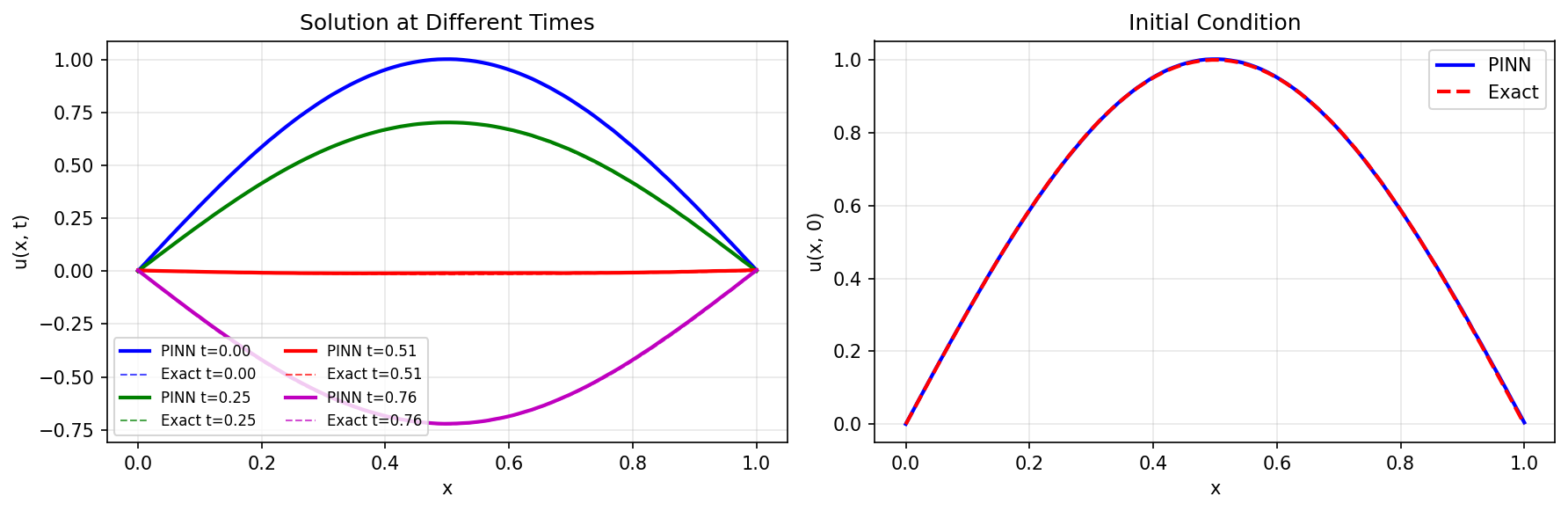
Initial position	\(u(x, 0) = \sin(\pi x)\)
Initial velocity	\(\frac{\partial u}{\partial t}(x, 0) = 0\)
Boundary conditions	\(u(0, t) = u(1, t) = 0\) (fixed ends)
Analytical solution	\(u(x, t) = \sin(\pi x) \cos(c\pi t)\)

Physical Interpretation¶

Standing wave: The initial condition \(\sin(\pi x)\) with zero velocity creates a standing wave
Fixed boundaries: String endpoints are held fixed (Dirichlet conditions)
Oscillation: The solution oscillates in time with frequency \(c\pi\)

PINN Loss Components¶

graph TB
    subgraph Input["Collocation Points"]
        A["Domain Points<br/>(x, t) in Ω"]
        B["Boundary Points<br/>x=0, x=1"]
        C["Initial Points<br/>t=0"]
    end

    subgraph PINN["Neural Network u_θ(x, t)"]
        D["Linear + tanh<br/>50 units"]
        E["Linear + tanh<br/>50 units"]
        F["Linear + tanh<br/>50 units"]
        G["Linear<br/>1 unit"]
    end

    subgraph Loss["Physics-Informed Loss"]
        H["PDE Residual<br/>|u_tt - c²u_xx|²"]
        I["BC Loss<br/>|u(0,t)|² + |u(1,t)|²"]
        J["IC Position<br/>|u(x,0) - sin(πx)|²"]
        K["IC Velocity<br/>|u_t(x,0)|²"]
        L["Total Loss"]
    end

    A --> D --> E --> F --> G --> H
    B --> D
    C --> D
    G --> I
    G --> J
    G --> K
    H --> L
    I --> L
    J --> L
    K --> L

    style H fill:#e3f2fd,stroke:#1976d2
    style I fill:#fff3e0,stroke:#f57c00
    style J fill:#e8f5e9,stroke:#388e3c
    style K fill:#fce4ec,stroke:#c2185b
    style L fill:#f3e5f5,stroke:#7b1fa2

Implementation¶

Step 1: Imports and Configuration¶

import jax
import jax.numpy as jnp
import optax
from flax import nnx

Terminal Output:

======================================================================
Opifex Example: Wave Equation PINN
======================================================================
JAX backend: gpu
JAX devices: [CudaDevice(id=0)]
Wave speed: c = 1.0
Domain: x in [0.0, 1.0], t in [0.0, 1.0]
Collocation: 2000 domain, 200 boundary, 200 initial
Network: [2] + [50, 50, 50] + [1]
Training: 15000 epochs @ lr=0.001

Step 2: Define the Problem¶

C = 1.0  # Wave speed

def exact_solution(x, t):
    return jnp.sin(jnp.pi * x) * jnp.cos(C * jnp.pi * t)

def initial_condition(x):
    return jnp.sin(jnp.pi * x)

Terminal Output:

Wave equation: u_tt = c^2 * u_xx
Initial condition: u(x, 0) = sin(pi*x)
Initial velocity: u_t(x, 0) = 0
Boundary conditions: u(0, t) = u(1, t) = 0
Analytical solution: u(x, t) = sin(pi*x) * cos(c*pi*t)

Step 3: Create the PINN¶

class WavePINN(nnx.Module):
    def __init__(self, hidden_dims: list[int], *, rngs: nnx.Rngs):
        layers = []
        in_features = 2  # (x, t)

        for hidden_dim in hidden_dims:
            layers.append(nnx.Linear(in_features, hidden_dim, rngs=rngs))
            in_features = hidden_dim

        layers.append(nnx.Linear(in_features, 1, rngs=rngs))
        self.layers = nnx.List(layers)

    def __call__(self, xt):
        h = xt
        for layer in self.layers[:-1]:
            h = jnp.tanh(layer(h))
        return self.layers[-1](h)

pinn = WavePINN(hidden_dims=[50, 50, 50], rngs=nnx.Rngs(42))

Terminal Output:

Creating PINN model...
PINN parameters: 5,301

Step 4: Compute PDE Residual¶

def compute_pde_residual(pinn, xt):
    def u_scalar(xt_single):
        return pinn(xt_single.reshape(1, 2)).squeeze()

    def residual_single(xt_single):
        hess = jax.hessian(u_scalar)(xt_single)
        u_xx = hess[0, 0]  # d^2u/dx^2
        u_tt = hess[1, 1]  # d^2u/dt^2
        return u_tt - C**2 * u_xx

    return jax.vmap(residual_single)(xt)

Step 5: Training¶

Terminal Output:

Training PINN...
  Epoch     1/15000: loss=4.347104e+00
  Epoch  3000/15000: loss=1.659206e-03
  Epoch  6000/15000: loss=1.217277e-03
  Epoch  9000/15000: loss=8.646434e-04
  Epoch 12000/15000: loss=3.246390e-04
  Epoch 15000/15000: loss=9.056964e-04
Final loss: 9.056964e-04

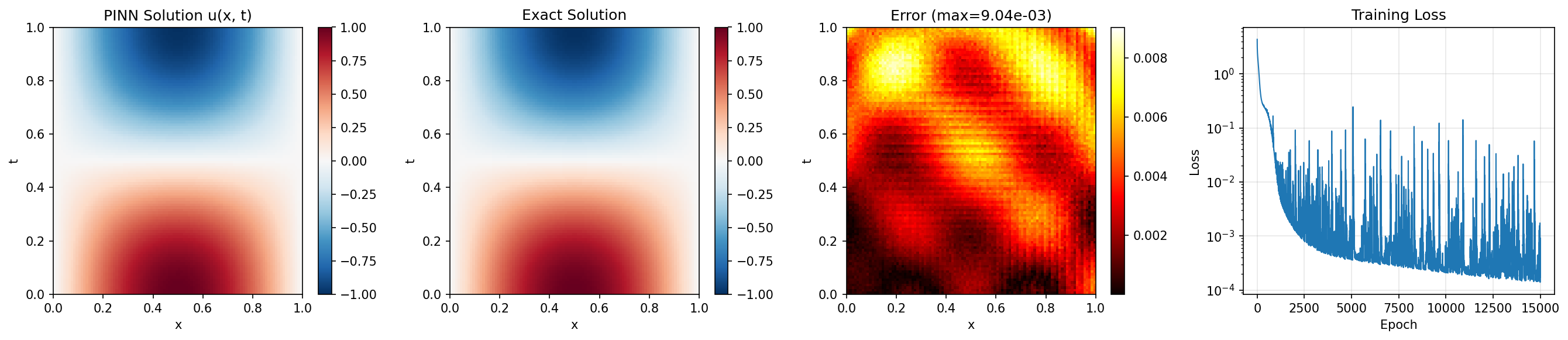
Step 6: Evaluation¶

Terminal Output:

Evaluating PINN...
Relative L2 error:   8.166147e-03
Maximum point error: 9.041926e-03
Mean point error:    3.580939e-03
Mean PDE residual:   7.680781e-03

Visualization¶

Solution Comparison¶

Wave Equation Solution

Time Snapshots¶

Analysis

Results Summary¶

Metric	Value
Final Loss	9.06e-04
Relative L2 Error	0.82%
Maximum Point Error	9.04e-03
Mean Point Error	3.58e-03
Mean PDE Residual	7.68e-03
Parameters	5,301
Training Epochs	15,000

Next Steps¶

Experiments to Try¶

Higher wave speed: Try \(c = 2\) or \(c = 5\) (faster oscillations)
Traveling wave: Change IC to \(u(x, 0) = e^{-(x-0.5)^2/0.01}\) Gaussian pulse
Longer time: Extend \(t_{max}\) to observe multiple oscillations
More modes: Try IC \(u(x,0) = \sin(\pi x) + 0.5\sin(2\pi x)\) for superposition
Damped wave: Add damping term \(-\gamma u_t\) to the PDE

Example	Level	What You'll Learn
Heat Equation	Intermediate	Parabolic PDE (diffusion)
Burgers Equation	Intermediate	Nonlinear hyperbolic PDE
Poisson Equation	Intermediate	Elliptic PDE (steady-state)
Helmholtz Equation	Advanced	Wave equation in frequency domain

API Reference¶

nnx.Linear - Linear layer
nnx.Optimizer - Optimizer wrapper
jax.hessian - Hessian computation
jax.vmap - Vectorized mapping

Troubleshooting¶

Solution doesn't oscillate¶

Symptom: PINN solution decays to zero instead of oscillating.

Cause: Initial velocity condition not enforced strongly enough.

Solution: Increase the weight on the initial velocity loss:

def total_loss(pinn, xt_dom, xt_bc, xt_ic, u_ic, lambda_ic=20.0):
    loss_pde = pde_loss(pinn, xt_dom)
    loss_bc = boundary_loss(pinn, xt_bc)
    loss_ic = initial_loss(pinn, xt_ic, u_ic)
    loss_vel = initial_velocity_loss(pinn, xt_ic)
    return loss_pde + 10 * loss_bc + lambda_ic * (loss_ic + 2.0 * loss_vel)

High error at later times¶

Symptom: Error grows as \(t\) increases.

Cause: Wave propagation is poorly captured far from initial conditions.

Solution: Use more collocation points or time-stratified sampling:

# Stratify points uniformly across time
t_domain = jnp.linspace(T_MIN, T_MAX, N_DOMAIN)
x_domain = jax.random.uniform(key, (N_DOMAIN,), minval=X_MIN, maxval=X_MAX)

Loss doesn't decrease¶

Symptom: Training loss stays constant or oscillates.

Cause: Network unable to satisfy competing constraints simultaneously.

Solution: Use adaptive loss weighting:

# Adjust weights based on individual loss magnitudes
loss_pde_val = pde_loss(pinn, xt_domain)
loss_bc_val = boundary_loss(pinn, xt_boundary)
loss_ic_val = initial_loss(pinn, xt_initial, u_initial)

# Normalize to similar magnitudes
weight_bc = loss_pde_val / (loss_bc_val + 1e-8)
weight_ic = loss_pde_val / (loss_ic_val + 1e-8)

Spectral bias issues¶

Symptom: Network captures low-frequency modes but misses high-frequency details.

Cause: Neural networks naturally favor low-frequency solutions (spectral bias).

Solution: Use Fourier feature encoding:

def fourier_features(xt, scales=[1, 2, 4]):
    features = [xt]
    for s in scales:
        features.append(jnp.sin(2 * jnp.pi * s * xt))
        features.append(jnp.cos(2 * jnp.pi * s * xt))
    return jnp.concatenate(features, axis=-1)

Wave Equation PINN¶

Overview¶

What You'll Learn¶

Coming from DeepXDE?¶

Files¶

Quick Start¶

Run the Python Script¶

Run the Jupyter Notebook¶

Core Concepts¶

Wave Equation¶

Physical Interpretation¶

PINN Loss Components¶

Implementation¶

Step 1: Imports and Configuration¶

Step 2: Define the Problem¶

Step 3: Create the PINN¶

Step 4: Compute PDE Residual¶

Step 5: Training¶

Step 6: Evaluation¶

Visualization¶

Solution Comparison¶

Time Snapshots¶

Results Summary¶

Next Steps¶

Experiments to Try¶

Related Examples¶

API Reference¶

Troubleshooting¶

Solution doesn't oscillate¶

High error at later times¶

Loss doesn't decrease¶

Spectral bias issues¶