Neural Operator Comparison Tour

Metadata	Value
Level	Advanced
Runtime	~10 min (CPU), ~3 min (GPU)
Prerequisites	JAX, Flax NNX, Neural Operators
Format	Python + Jupyter

Overview

This example tours the Fourier-family neural operators in Opifex and runs a fair, head-to-head comparison of them on a single Darcy-flow benchmark. Every operator is trained with the same recipe -- grid positional embedding, Gaussian input/output normalization, the relative-L2 loss, and an identical optimizer budget -- so the resulting accuracy and parameter counts are directly comparable.

Unlike single-model tutorials, this demo maps the trade-offs across the opifex.neural.operators Fourier family. Each operator maps a high-contrast permeability field a(x) ∈ {3, 12} to the Darcy pressure solution of -∇·(a∇u) = 1. We report the test relative-L2 error, the parameter count, and the training time, then visualise the trade-offs.

What You'll Learn

1. Discover operators with list_operators() and recommend_operator()
2. Apply one recipe uniformly across Dense FNO, Tucker/CP Tensorized FNO, Local FNO, and U-FNO
3. Read a fair accuracy-vs-parameters comparison on real Darcy data
4. Understand the Tucker/CP compression trade-off against a dense FNO
5. Validate against a floor -- every operator must beat a mean predictor

Coming from NeuralOperator (PyTorch)?

If you are familiar with the neuraloperator library, here is how Opifex compares for this workflow:

NeuralOperator (PyTorch)	Opifex (JAX)
FNO(n_modes, hidden_channels)	FourierNeuralOperator(modes=, hidden_channels=, num_layers=, positional_embedding=True, rngs=)
TFNO(n_modes, hidden_channels, factorization)	create_tucker_fno(modes=, hidden_channels=, rank=, rngs=) / create_cp_fno(...)
Local FNO with manual conv branches	LocalFourierNeuralOperator(modes=, hidden_channels=, num_layers=, rngs=)
UNO(...) with manual U-Net wiring	UFourierNeuralOperator(modes=, hidden_channels=, num_levels=, rngs=)
No built-in operator factory	create_operator("SFNO", ...) and recommend_operator("global_climate")
torch.optim.Adam(model.parameters(), lr)	optax.adam(lr) (handled internally by Trainer)

Key differences:

1. Explicit PRNG: Opifex uses JAX's explicit rngs=nnx.Rngs(42) instead of global random state
2. Factory system: create_operator() and recommend_operator() provide guided operator selection
3. XLA compilation: All forward passes are JIT-compiled automatically for hardware acceleration
4. Functional transforms: jax.grad, jax.vmap, jax.pmap compose cleanly with every operator variant

Files

• Python Script: examples/neural-operators/operator_tour.py
• Jupyter Notebook: examples/neural-operators/operator_tour.ipynb

Quick Start

Run the Python Script

source activate.sh && python examples/neural-operators/operator_tour.py

Run the Jupyter Notebook

jupyter lab examples/neural-operators/operator_tour.ipynb

Core Concepts

The Fourier Operator Family

Opifex provides a unified framework where every Fourier-family operator shares the same (in_channels, out_channels, hidden_channels, modes, rngs) interface and the same channels-first (batch, channels, height, width) data layout. This tour compares five of them.

Operator	Full Name	Distinguishing Feature
Dense FNO	Fourier Neural Operator	Full (dense) spectral weights; the baseline
Tucker TFNO	Tucker-Tensorized FNO	Spectral weights stored as a Tucker factorization
CP TFNO	CP-Tensorized FNO	Spectral weights stored as a CP factorization (most compact)
Local FNO	Local Fourier Neural Operator	Adds local convolution branches to the spectral path
U-FNO	U-Net Fourier Neural Operator	Multi-scale encoder-decoder over spectral blocks

Operator Discovery System

The factory system provides three entry points:

• list_operators() -- returns all available operators grouped by category
• recommend_operator(application) -- suggests the best operator for a given application
• create_operator(name, **kwargs) -- instantiates any operator by name

The Shared Recipe (Fair Comparison)

The comparison is only meaningful if every operator is given the same chance. We apply the proven operator-learning recipe identically:

• Grid positional embedding -- FNO and the Tensorized FNOs append normalized (x, y) coordinate channels internally; Local FNO and U-FNO are wrapped so they receive the same channels.
• Gaussian normalization of inputs and outputs, fit on the training split.
• Relative-L2 loss via LossConfig(loss_type="relative_l2").
• Identical budget -- 1024 train samples, 100 epochs, Adam at 1e-3.

Implementation

Step 1: Imports and Setup

import time
import warnings
from pathlib import Path
from typing import Any

warnings.filterwarnings("ignore")

import jax
import jax.numpy as jnp
import matplotlib as mpl
import numpy as np
from flax import nnx

mpl.use("Agg")
import matplotlib.pyplot as plt

from opifex.core.training import Trainer, TrainingConfig
from opifex.core.training.config import LossConfig
from opifex.data.loaders import create_darcy_loader
from opifex.neural.operators import (
    FourierNeuralOperator,
    LocalFourierNeuralOperator,
    UFourierNeuralOperator,
    list_operators,
    recommend_operator,
)
from opifex.neural.operators.fno._positional import append_grid_coordinates
from opifex.neural.operators.fno.tensorized import create_cp_fno, create_tucker_fno

Terminal Output:

======================================================================
Opifex Example: Neural Operator Comparison Tour on Darcy Flow
======================================================================
JAX backend: gpu
JAX devices: [CudaDevice(id=0)]
Resolution: 64x64
Training samples: 1024, Test samples: 256
Shared FNO config: modes=16, width=32, layers=4

Step 2: Operator Discovery

The factory lists every available operator by category and recommends one per application domain.

for category, operators in list_operators().items():
    print(f"  {category}: {', '.join(operators)}")

applications = [
    "turbulent_flow", "global_climate", "molecular_dynamics",
    "cad_geometry", "safety_critical", "parameter_efficient",
]
for app in applications:
    rec = recommend_operator(app)
    print(f"  {app:20s}: {rec['primary']} - {rec['reason']}")

Terminal Output:

======================================================================
OPERATOR DISCOVERY
======================================================================
Available operators by category:
  fourier_operators: FNO, TFNO, UFNO, SFNO, LocalFNO, AM-FNO
  deeponet_family: DeepONet, FourierDeepONet, AdaptiveDeepONet
  graph_operators: GNO, MGNO
  uncertainty_aware: FNO, DeepONet, PINO, TFNO, UFNO, SFNO, LocalFNO, AM-FNO, MS-FNO, FourierDeepONet, AdaptiveDeepONet, MultiPhysicsDeepONet, GINO, MGNO, UQNO, LNO, WNO, GNO, OperatorNet
  adapter_capable: FNO, DeepONet, PINO, TFNO, UFNO, SFNO, LocalFNO, AM-FNO, MS-FNO, FourierDeepONet, AdaptiveDeepONet, MultiPhysicsDeepONet, GINO, MGNO, UQNO, LNO, WNO, GNO, OperatorNet
  geometry_aware: GINO, GNO, MGNO
  parameter_efficient: TFNO, LNO

Recommendations by application:
  turbulent_flow      : UFNO - Multi-scale encoder-decoder for turbulent structures
  global_climate      : SFNO - Spherical harmonics for global atmospheric modeling
  molecular_dynamics  : MGNO - Multipole expansion for long-range molecular interactions
  cad_geometry        : GINO - Geometry-aware processing for complex CAD shapes
  safety_critical     : UQNO - Uncertainty quantification for safety-critical decisions
  parameter_efficient : TFNO - Tensor factorization for memory efficiency

Step 3: Data Loading and Normalization

The Darcy loader generates a binary high-contrast permeability field and the exact pressure solution. A single create_darcy_loader(...) call returns a frozen PDELoaders with .train and .val datarax pipelines, split by val_fraction. We drain each pipeline into channels-first arrays and fit Gaussian statistics on the training set.

n_samples = N_TRAIN + N_TEST
loaders = create_darcy_loader(
    n_samples=n_samples,
    batch_size=BATCH_SIZE,
    resolution=RESOLUTION,
    field_type="binary",
    coeff_range=PERMEABILITY_VALUES,
    val_fraction=N_TEST / n_samples,
    seed=SEED,
)

X_train, Y_train = collect_darcy_split(loaders.train)
X_test, Y_test = collect_darcy_split(loaders.val)
# ... fit Gaussian statistics and normalize ...
x_mean, x_std = X_train.mean(), X_train.std()
y_mean, y_std = Y_train.mean(), Y_train.std()
X_train_n = jnp.array((X_train - x_mean) / x_std)
Y_train_n = jnp.array((Y_train - y_mean) / y_std)

The collect_darcy_split helper drains a datarax pipeline into channels-first (N, 1, H, W) arrays:

def collect_darcy_split(pipeline: Any) -> tuple[np.ndarray, np.ndarray]:
    """Drain a datarax pipeline into channels-first ``(N, 1, H, W)`` arrays."""
    inputs, outputs = [], []
    for batch in pipeline:
        inputs.append(np.asarray(batch["input"]))
        outputs.append(np.asarray(batch["output"]))
    return np.concatenate(inputs, axis=0), np.concatenate(outputs, axis=0)

Terminal Output:

Generating Darcy flow data...
Training data: X=(1024, 1, 64, 64), Y=(1024, 1, 64, 64)
Test data:     X=(256, 1, 64, 64), Y=(256, 1, 64, 64)
Input mean/std:  7.4976 / 4.5000
Output mean/std: 0.005354 / 0.003583

Step 4: Building the Comparison Set

All five operators map (batch, 1, H, W) permeability to pressure. Local FNO and U-FNO are wrapped so they receive the same grid-coordinate channels as the FNO / TFNO family -- the only difference between models is the architecture.

class GridWrapped(nnx.Module):
    """Append grid coordinates before applying an operator without built-in embedding."""

    def __init__(self, operator: nnx.Module) -> None:
        super().__init__()
        self.operator = operator

    def __call__(self, x: jax.Array) -> jax.Array:
        return self.operator(append_grid_coordinates(x))


grid_in_channels = 1 + 2  # permeability + (x, y) coordinate channels
operators = {
    "Dense FNO": FourierNeuralOperator(
        in_channels=1, out_channels=1, hidden_channels=HIDDEN_CHANNELS,
        modes=MODES, num_layers=NUM_LAYERS, positional_embedding=True,
        rngs=nnx.Rngs(SEED),
    ),
    "Tucker TFNO": create_tucker_fno(
        in_channels=1, out_channels=1, hidden_channels=HIDDEN_CHANNELS,
        modes=(MODES, MODES), rank=TUCKER_RANK, num_layers=NUM_LAYERS,
        rngs=nnx.Rngs(SEED + 1),
    ),
    "CP TFNO": create_cp_fno(
        in_channels=1, out_channels=1, hidden_channels=HIDDEN_CHANNELS,
        modes=(MODES, MODES), rank=CP_RANK, num_layers=NUM_LAYERS,
        rngs=nnx.Rngs(SEED + 2),
    ),
    "Local FNO": GridWrapped(LocalFourierNeuralOperator(
        in_channels=grid_in_channels, out_channels=1, hidden_channels=HIDDEN_CHANNELS,
        modes=(MODES, MODES), num_layers=NUM_LAYERS, rngs=nnx.Rngs(SEED + 3),
    )),
    "U-FNO": GridWrapped(UFourierNeuralOperator(
        in_channels=grid_in_channels, out_channels=1, hidden_channels=HIDDEN_CHANNELS,
        modes=(MODES, MODES), num_levels=UFNO_LEVELS, rngs=nnx.Rngs(SEED + 4),
    )),
}

Terminal Output:

Comparison operators (parameter counts):
  Dense FNO     : 4,203,009 params
  Tucker TFNO   : 150,017 params
  CP TFNO       : 14,913 params
  Local FNO     : 610,859 params
  U-FNO         : 6,994,881 params

Tensorized FNO Compression

The dense FNO uses full spectral weights, while the Tucker and CP factorized FNOs store the same spectral operators in low-rank form. At rank=0.5 the Tucker TFNO is 28x smaller and the CP TFNO is 282x smaller than the dense FNO -- and on this benchmark they stay within a hair of its accuracy.

Step 5: Training Each Operator

Every operator reuses the same Trainer configuration: Adam at 1e-3, the relative-L2 loss, and 100 epochs. Only the architecture changes between runs.

config = TrainingConfig(
    num_epochs=100, learning_rate=1e-3, batch_size=32,
    validation_frequency=10, verbose=False,
    loss_config=LossConfig(loss_type="relative_l2"),
)
trainer = Trainer(model=model, config=config, rngs=nnx.Rngs(42))
trained_model, metrics = trainer.fit(
    train_data=(X_train_n, Y_train_n),
    val_data=(X_test_n, Y_test_n),
)
# Un-normalize predictions before measuring physical-space relative L2
predictions = predict_in_batches(trained_model, X_test_n) * y_std + y_mean

Terminal Output:

======================================================================
TRAINING COMPARISON
======================================================================

----------------------------------------------------------------------
Training Dense FNO (4,203,009 params)...
  Dense FNO: rel-L2=0.0177, MSE=1.404e-08, time=13.2s, final val loss=0.0016

----------------------------------------------------------------------
Training Tucker TFNO (150,017 params)...
  Tucker TFNO: rel-L2=0.0183, MSE=1.433e-08, time=13.8s, final val loss=0.0010

----------------------------------------------------------------------
Training CP TFNO (14,913 params)...
  CP TFNO: rel-L2=0.0253, MSE=2.778e-08, time=13.5s, final val loss=0.0026

----------------------------------------------------------------------
Training Local FNO (610,859 params)...
  Local FNO: rel-L2=0.0367, MSE=5.626e-08, time=19.0s, final val loss=0.0049

----------------------------------------------------------------------
Training U-FNO (6,994,881 params)...
  U-FNO: rel-L2=0.0293, MSE=3.993e-08, time=32.6s, final val loss=0.0028

Step 6: Mean-Predictor Floor

A fair comparison needs a floor. The mean predictor always outputs the training mean pressure -- any operator worth using must beat it.

mean_field = jnp.full_like(Y_test_jnp, float(Y_train.mean()))
mean_baseline_rel_l2 = float(jnp.mean(relative_l2(mean_field, Y_test_jnp)))

Terminal Output:

Mean-predictor relative-L2: 0.5576
Every trained operator must beat this floor to be useful.

Results Summary

Terminal Output:

======================================================================
COMPARISON SUMMARY (sorted by relative-L2)
======================================================================

Operator          Rel-L2         MSE      Params   vs FNO   Time(s)
-------------------------------------------------------------------
Dense FNO         0.0177   1.404e-08   4,203,009    1.00x      13.2
Tucker TFNO       0.0183   1.433e-08     150,017   28.02x      13.8
CP TFNO           0.0253   2.778e-08      14,913  281.84x      13.5
U-FNO             0.0293   3.993e-08   6,994,881    0.60x      32.6
Local FNO         0.0367   5.626e-08     610,859    6.88x      19.0
Mean predictor    0.5576

Best accuracy: Dense FNO (rel-L2=0.0177)

Comparison Table

Operator	Test Rel-L2	Test MSE	Parameters	Size vs Dense FNO
Dense FNO	0.0177	1.404e-08	4,203,009	1.00x (baseline)
Tucker TFNO	0.0183	1.433e-08	150,017	28.02x smaller
CP TFNO	0.0253	2.778e-08	14,913	281.84x smaller
U-FNO	0.0293	3.993e-08	6,994,881	0.60x (larger)
Local FNO	0.0367	5.626e-08	610,859	6.88x smaller
Mean predictor	0.5576	--	--	--

Predictions (Best Operator)

The most accurate operator (Dense FNO) recovers the Darcy pressure field with a small absolute error concentrated near the high-contrast permeability interfaces.

Accuracy, Size, and Cost

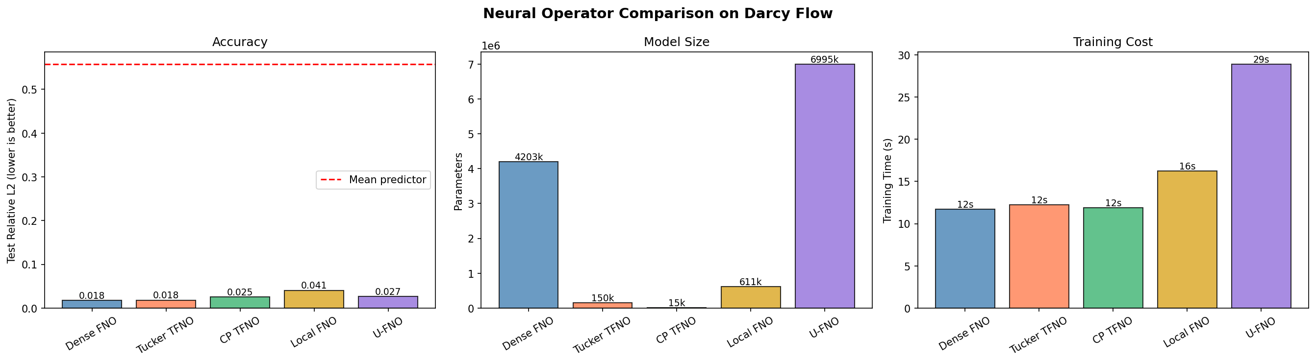
The three bar charts summarise the trade-offs: test accuracy (lower is better), parameter count (lower is more efficient), and training time.

What We Achieved

• Trained five Fourier-family operators on the same Darcy benchmark with the same recipe, so accuracy and size are directly comparable
• Established a clear floor: every operator beats the mean predictor (0.5576) by more than an order of magnitude
• Demonstrated the Tensorized FNO compression story -- the Tucker TFNO matches the dense FNO's accuracy (0.0183 vs 0.0177) at 28x fewer parameters, and the CP TFNO stays competitive (0.0253) at 282x fewer parameters
• Verified that Local FNO and U-FNO learn the operator competitively when given the same grid-embedding recipe

Next Steps

Experiments to Try

1. Sweep the factorization rank: Try Tucker / CP rank of 0.25, 0.5, 0.75 to map the accuracy-compression curve
2. Add Tensor-Train: Compare create_tt_fno() against Tucker and CP
3. Increase capacity: Raise hidden_channels, modes, or num_layers
4. Specialized operators: Apply SFNO, GINO, MGNO, or UQNO on their native domains (climate, geometry, molecules, uncertainty)
5. Use the factory: Let recommend_operator() guide architecture selection for new problem domains

Related Examples

Example	Level	What You'll Learn
FNO on Darcy Flow	Intermediate	Standard FNO training pipeline on Darcy flow
TFNO on Darcy Flow	Intermediate	The Tucker compression story in depth
UNO on Darcy Flow	Intermediate	Multi-resolution U-shaped neural operator
Local FNO on Darcy Flow	Intermediate	Combined local + global Fourier operations
Grid Embeddings	Beginner	Spatial coordinate injection for neural operators

API Reference

• FourierNeuralOperator -- Dense FNO with spectral convolution layers
• create_tucker_fno -- Tucker-factorized (Tensorized) FNO
• create_cp_fno -- CP-factorized (Tensorized) FNO
• LocalFourierNeuralOperator -- Local FNO with conv + spectral branches
• UFourierNeuralOperator -- U-FNO with multi-scale encoder-decoder
• create_operator -- Factory function for creating any operator by name
• recommend_operator -- Application-aware operator recommendation
• list_operators -- List all available operators by category

Troubleshooting

An operator does not beat the mean predictor

Symptom: A trained operator's relative-L2 is near 0.5576 (the mean-predictor floor).

Cause: The model is not learning -- usually a missing positional embedding or un-normalized targets.

Solution: Confirm the input carries grid coordinates (built in for FNO / TFNO, added by GridWrapped for Local FNO / U-FNO), that inputs and outputs are Gaussian-normalized, and that the loss is relative_l2.

OOM during training

Symptom: RESOURCE_EXHAUSTED when training the larger operators (U-FNO).

Cause: U-FNO with num_levels=3 and hidden_channels=32 doubles channels per level, so it is the largest model in the tour.

Solution: Reduce HIDDEN_CHANNELS, lower UFNO_LEVELS, or shrink BATCH_SIZE.

Slow first epoch

Symptom: The first epoch of each operator is much slower than the rest.

Cause: The first forward/backward pass triggers XLA compilation. Subsequent steps reuse the compiled program.

Solution: This is expected; the reported training times already include compilation. Run on GPU for the fastest turnaround. ```