Learn-to-Optimize (L2O): A Meta-Trained Optimiser for Neural-Network Training

Level	Runtime	Prerequisites	Format	Memory
Intermediate	~25 s (GPU)	JAX basics, gradient-based optimisation	Tutorial	~1 GB

Overview

This example meta-trains a learned optimiser — a small neural network that is an optimiser update rule — and shows it generalising to held-out neural-network training problems where it beats a properly tuned classical optimiser.

A hand-designed optimiser (SGD, Adam) applies the same fixed update rule to every problem. A learned optimiser is trained so that its update rule is itself good across a whole distribution of objectives. Opifex follows the design of Google's learned_optimization library and the L2O literature.

Key insight: L2O's genuine advantage shows on non-convex, stochastic training — where a single fixed learning rate is most compromised and the learned optimiser's implicit learning-rate schedule (a tanh embedding of the step index) gives it a real edge. The showcase task here is therefore small neural-network training, not a convex toy.

What You'll Learn

1. Tasks carry their objective — Task / TaskFamily provide a meta-training distribution and a held-out meta-test split.
2. A per-parameter MLP optimiser — MLPLearnedOptimizer maps per-parameter features to a (direction, magnitude) update, shared across all coordinates.
3. PES meta-training — Persistent Evolution Strategies meta-trains the optimiser without back-propagating through the unroll.
4. Honest benchmarking — compare against distribution-tuned Adam and SGD on held-out tasks and report speedup-at-target, scoped to in-distribution generalisation.

Files

• Python script: examples/optimization/learn_to_optimize.py
• Jupyter notebook: examples/optimization/learn_to_optimize.ipynb

Quick Start

Run the script

source activate.sh && python examples/optimization/learn_to_optimize.py

Run the notebook

source activate.sh && jupyter lab examples/optimization/learn_to_optimize.ipynb

Background

• Andrychowicz et al. 2016, Learning to learn by gradient descent by gradient descent (arXiv:1606.04474).
• Metz et al. 2020, Tasks, stability, architecture, and compute (arXiv:2009.11243) — the per-parameter MLP optimiser.
• Vicol et al. 2021, Persistent Evolution Strategies (arXiv:2112.13835) — the meta-training estimator.
• Eldan et al. 2023 (arXiv:2310.18191) — the cautionary critique on out-of-distribution generalisation, which is why every claim below is scoped to held-out tasks from the meta-training family.

See Learn-to-Optimize Methods for the full method description.

Implementation

Step 1: A family of small neural-network training tasks

Each task is a teacher-student MLP regression: a random teacher MLP generates targets from Gaussian inputs, and the student (same architecture) is trained by MSE on stochastic minibatches. The optimum (loss 0) is realisable, but the landscape is non-convex in the student weights — the genuine L2O setting. A fresh teacher and dataset per task force the meta-trained optimiser to generalise across many training problems.

from opifex.optimization.l2o import L2OEngine, MLPLearnedOptimizer, MLPTaskFamily

family = MLPTaskFamily(
    input_dim=8, hidden_dim=16, output_dim=4, num_data=512, batch_size=32
)
learned_optimizer = MLPLearnedOptimizer(hidden_size=32, hidden_layers=2, step_mult=0.03)
engine = L2OEngine(learned_optimizer, family)

Terminal Output:

Building MLP task family and learned optimiser...
------------------------------------------------------------------------
  Inner task: teacher-student MLP 8->16->4 (MSE)
  Tasks per PES step: 32
  Learned optimiser: per-parameter MLP (32x2), 19 input features

Step 2: Meta-train the learned optimiser with PES

L2OEngine.meta_train runs Persistent Evolution Strategies: it perturbs the optimiser meta-parameters antithetically, unrolls the inner training on 32 tasks in parallel, and feeds the unbiased ES gradient estimate to an outer Adam. The whole inner unroll is JIT-compiled and scanned — there is no Python-level optimisation loop.

meta_losses = engine.meta_train(
    jax.random.key(0),
    num_outer_steps=3000, num_tasks=32,
    trunc_length=20, total_horizon=100,
    perturbation_std=0.01, meta_learning_rate=3e-3,
)

Terminal Output:

Meta-training with PES...
------------------------------------------------------------------------
  Outer steps: 3000
  Meta-loss (first 20 steps avg): 1.1082
  Meta-loss (last 20 steps avg):  0.0929
  Meta-loss reduction: 11.93x

Step 3: Meta-test on a held-out split vs tuned Adam and SGD

The trained optimiser is applied to 48 fresh tasks (a different RNG stream = in-distribution held-out split) and compared against distribution-tuned Adam and SGD baselines: a single learning rate is selected on the task distribution and applied unchanged to every held-out task (a per-task sweep would be an undeployable oracle). The speedup is measured at a per-task target loss (10% of the baseline's initial loss), censoring any task that never reaches it.

adam_result = engine.benchmark(
    jax.random.key(1), num_tasks=48, num_steps=100,
    target_fraction=0.1, transformation=optax.adam,
)
sgd_result = engine.benchmark(
    jax.random.key(2), num_tasks=48, num_steps=100,
    target_fraction=0.1, transformation=optax.sgd,
)

Terminal Output:

Meta-testing on held-out tasks vs distribution-tuned baselines...
------------------------------------------------------------------------
  Held-out tasks: 48
  Learned final loss (mean):    1.6052
  Tuned-Adam final loss (mean): 1.8185 (lr=0.100)
  Tuned-SGD final loss (mean):  2.7426 (lr=0.100)
  Median speedup @ 10%-target vs tuned Adam: 1.82x
  Median speedup @ 10%-target vs tuned SGD:  2.67x

Results

========================================================================
RESULTS SUMMARY
========================================================================
  Meta-loss reduction:            11.93x
  Learned final loss (held-out):  1.6052
  Tuned-Adam final loss:          1.8185
  Tuned-SGD final loss:           2.7426
  Speedup vs tuned Adam:          1.82x
  Speedup vs tuned SGD:           2.67x
========================================================================

The meta-trained optimiser decisively beats tuned SGD (≈2.7× faster to the target, lower final loss) and beats tuned Adam (≈1.8× faster, lower final loss) on held-out tasks — and it trains in ~25 s on a GPU. The claim is scoped to held-out tasks drawn from the meta-training family; it is not an out-of-distribution result (cf. arXiv:2310.18191).

Method	Held-out final loss (mean)	Speedup @ 10%-target
Learned (L2O)	1.61	—
Tuned Adam	1.82	1.82× (learned is faster)
Tuned SGD	2.74	2.67× (learned is faster)

Visualization

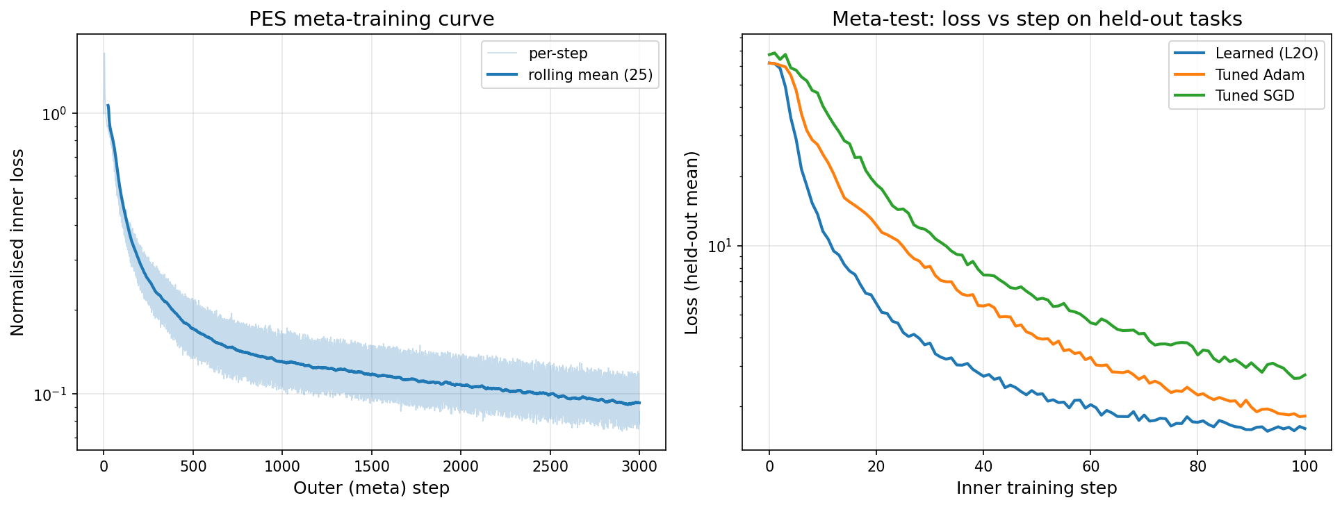
Meta-training curve and held-out learning curves

The left panel is the PES meta-training curve (raw per-step loss faint, rolling-mean trend bold — the standard presentation for an evolution-strategies estimate). The right panel is the meta-test: the learned optimiser (blue) descends below tuned Adam (orange) and tuned SGD (green) on held-out tasks.

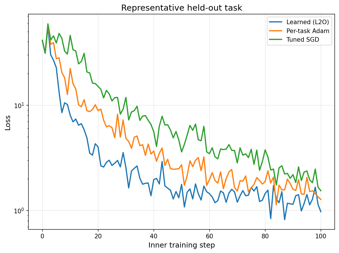
Representative held-out task

A single held-out task: the learned optimiser versus per-task-tuned Adam and tuned SGD.

Next Steps

Experiments to Try

• Increase num_outer_steps or num_tasks for a stronger learned optimiser (PES variance drops with more parallel tasks).
• Vary the task family (hidden_dim, num_data, batch_size) and watch generalisation change.
• Swap in LearnableSGD to validate the PES estimator against a single learnable learning rate.
• Persist and reload the meta-learned parameters with engine.save_theta / engine.load_theta.

Related Examples

• Meta-Optimization — the opifex.optimization.meta_optimization framework.

API Reference

• Learn-to-Optimize Methods
• Optimization API

Troubleshooting

The meta-training curve is noisy

PES is an evolution-strategies estimator, so the per-step meta-loss is inherently noisy; the example overlays a rolling mean to show the trend. Increasing num_tasks lowers the variance.

Meta-training diverges

A too-large meta_learning_rate (outer Adam) or step_mult can destabilise PES — reduce them, or increase num_tasks (≥32 keeps PES stable for this task). The reference defaults (step_mult=1e-3) are calibrated for much longer training; this short demo uses step_mult=0.03.

The learned optimiser does not beat the baseline

Generalisation is scoped to held-out tasks from the meta-training family. A learned optimiser trained on one family is not expected to beat tuned baselines on a different distribution.