Full SFNO for Climate Modeling

Metadata	Value
Level	Advanced
Runtime	~10 min (CPU) / ~4 sec (GPU)
Prerequisites	JAX, Flax NNX, Spherical Harmonics, Conservation Laws
Format	Python + Jupyter
Memory	~2 GB RAM
Devices	CPU / GPU (GPU recommended)

Overview

This example demonstrates full Spherical Fourier Neural Operator (SFNO) functionality for climate modeling using the Opifex framework with JAX/Flax NNX. The SFNO extends the standard FNO to spherical geometries by replacing Fourier transforms with spherical harmonic transforms, making it the natural architecture for global climate and weather prediction tasks where data lives on the surface of a sphere.

The example covers the full pipeline: creating an SFNO model with create_climate_sfno, loading shallow water equation data via create_shallow_water_loader (Google Grain), training with conservation-aware physics loss through ConservationConfig, evaluating energy and mass conservation, and performing spherical harmonic spectral analysis of predictions.

Conservation-aware training is a key feature of this example. By configuring ConservationConfig with energy and mass conservation laws, the Trainer adds physics-informed loss terms that penalize violations of fundamental physical invariants -- ensuring the learned operator respects the underlying physics of climate dynamics.

What You'll Learn

1. Build an SFNO model with create_climate_sfno for spherical domain climate data
2. Configure conservation-aware training with ConservationConfig for energy and mass conservation
3. Analyze spherical harmonic power spectra to evaluate spectral fidelity of predictions
4. Evaluate energy and mass conservation metrics for physics-informed model quality
5. Visualize climate fields, error distributions, and spectral analysis on spherical domains

Coming from NeuralOperator (PyTorch)?

NeuralOperator (PyTorch)	Opifex (JAX)
SFNO(spectral_transform, ...)	create_climate_sfno(in_channels=, out_channels=, lmax=, rngs=)
SphericalConv(in_ch, out_ch, modes)	Spherical spectral convolution via lmax parameter
Manual conservation loss implementation	ConservationConfig(laws=["energy", "mass"]) built into Trainer
trainer.train(epochs=100)	Trainer(model, config, rngs).fit(train_data, val_data)
torch.DataLoader(dataset)	create_shallow_water_loader() (Google Grain)

Key differences:

1. Built-in conservation: Opifex integrates energy and mass conservation directly into the training loop via ConservationConfig, eliminating manual loss implementation
2. Factory functions: create_climate_sfno handles architecture configuration for climate applications
3. Explicit PRNG: JAX's rngs=nnx.Rngs(42) ensures reproducible model initialization
4. XLA compilation: Automatic JIT compilation provides training speedups on GPU/TPU

Coming from PhysicsNeMo (NVIDIA)?

PhysicsNeMo	Opifex (JAX)
FourierNeuralOperatorNet(cfg)	create_climate_sfno(in_channels=, out_channels=, lmax=, rngs=)
Hydra YAML for conservation config	ConservationConfig(laws=["energy", "mass"]) (pure Python)
Solver(cfg)	Trainer(model, config, rngs)
DistributedManager()	jax.devices(), automatic device management

Key differences:

1. No YAML required: Pure Python configuration vs mandatory Hydra config files
2. Simpler setup: No complex config directory structure needed
3. JAX ecosystem: Native integration with Flax, Optax, Grain

Files

• Python Script: examples/neural-operators/sfno_climate_comprehensive.py
• Jupyter Notebook: examples/neural-operators/sfno_climate_comprehensive.ipynb

Quick Start

Run the Python Script

source activate.sh && python examples/neural-operators/sfno_climate_comprehensive.py

Run the Jupyter Notebook

jupyter lab examples/neural-operators/sfno_climate_comprehensive.ipynb

Core Concepts

The Spherical Fourier Neural Operator

The SFNO adapts the FNO architecture to spherical geometry. Instead of standard 2D Fourier transforms, it uses spherical harmonic transforms (SHT) to operate in the spectral domain of the sphere. The lmax parameter controls the maximum spherical harmonic degree retained, analogous to modes in a standard FNO.

graph LR
    A["Climate Field<br/>on Sphere<br/>(lat x lon)"] --> B["Spherical Harmonics<br/>Transform (SHT)"]
    B --> C["Spectral Conv<br/>(learned weights<br/>up to degree lmax)"]
    C --> D["Inverse SHT"]
    A --> E["Local Linear<br/>(skip connection)"]
    D --> F["+ (Add)"]
    E --> F
    F --> G["Activation"]
    G --> H["Predicted<br/>Climate Field"]

    style A fill:#e3f2fd
    style H fill:#c8e6c9
    style C fill:#fff3e0

Each SFNO spectral layer consists of:

1. Spherical Harmonic Transform (SHT): Project the input field onto spherical harmonic basis functions \(Y_l^m(\theta, \phi)\)
2. Spectral convolution: Apply learned linear transforms to the spherical harmonic coefficients up to degree lmax
3. Inverse SHT: Transform back to the spatial (lat/lon) domain
4. Skip connection: Add a local linear transform of the input

Conservation-Aware Training

Climate models must respect fundamental physical conservation laws. Opifex's ConservationConfig adds physics-informed loss terms that penalize violations of energy and mass conservation during training.

flowchart TD
    subgraph Forward["Forward Pass"]
        A["Input Climate Field<br/>(shallow water data)"] --> B["SFNO Model<br/>create_climate_sfno()"]
    end

    subgraph Loss["Conservation-Aware Loss"]
        B --> C["Data Loss<br/>L_data = MSE(pred, target)"]
        B --> D["Energy Conservation<br/>L_energy = |E_pred - E_target|"]
        B --> E["Mass Conservation<br/>L_mass = |M_pred - M_target|"]
        C --> F["Total Loss<br/>L = L_data + lambda_E * L_energy + lambda_M * L_mass"]
        D --> F
        E --> F
    end

    subgraph Update["Parameter Update"]
        F --> G["jax.grad"]
        G --> H["Optimizer Step<br/>(optax Adam)"]
        H --> B
    end

    style A fill:#e3f2fd
    style F fill:#fff3e0
    style H fill:#c8e6c9

Shallow Water Equations

The shallow water equations (SWE) model large-scale geophysical fluid dynamics on the sphere. They form a standard benchmark for climate modeling architectures:

Variable	Meaning	Role
\(h\)	Fluid depth	Conserved quantity (mass)
\(u, v\)	Velocity components	Momentum carriers
\(E = \frac{1}{2}(u^2 + v^2 + gh^2)\)	Total energy	Conservation target

The 3-channel input/output (height + 2 velocity components) tests the SFNO's ability to learn coupled multi-field dynamics while preserving conservation properties.

Implementation

Step 1: Imports and Setup

import time
import warnings
from pathlib import Path

warnings.filterwarnings("ignore")

import jax
import jax.numpy as jnp
import matplotlib.pyplot as plt
import numpy as np
from flax import nnx

from opifex.core.training import ConservationConfig, Trainer, TrainingConfig
from opifex.data.loaders import create_shallow_water_loader
from opifex.neural.operators.fno.spherical import create_climate_sfno

Terminal Output:

======================================================================
Opifex Example: Full Spherical FNO for Climate Modeling
======================================================================
JAX backend: gpu
JAX devices: [CudaDevice(id=0)]

Device Support

This example works on both CPU and GPU. GPU is recommended for faster training. The JAX backend is detected automatically.

Step 2: Configuration

Define the key hyperparameters controlling the SFNO architecture and training:

RESOLUTION = 32
N_TRAIN = 200
N_TEST = 40
BATCH_SIZE = 8
NUM_EPOCHS = 5
LEARNING_RATE = 1e-3
LMAX = 8
IN_CHANNELS = 3
OUT_CHANNELS = 3
SEED = 42

OUTPUT_DIR = Path("docs/assets/examples/sfno_climate_comprehensive")
OUTPUT_DIR.mkdir(parents=True, exist_ok=True)

Terminal Output:

Resolution: 32x32, Samples: 200/40
Batch: 8, Epochs: 5, lmax: 8

Parameter	Value	Purpose
RESOLUTION	32	Spatial grid resolution (lat x lon)
LMAX	8	Maximum spherical harmonic degree
IN_CHANNELS / OUT_CHANNELS	3	Height + u-velocity + v-velocity
NUM_EPOCHS	5	Training iterations (increase for better accuracy)
LEARNING_RATE	1e-3	Adam optimizer step size

Step 3: Data Loading with Grain

Load shallow water equation data using Opifex's Grain-based data loader:

train_loader = create_shallow_water_loader(
    n_samples=N_TRAIN, batch_size=BATCH_SIZE, resolution=RESOLUTION,
    shuffle=True, seed=SEED + 3000, worker_count=0)
test_loader = create_shallow_water_loader(
    n_samples=N_TEST, batch_size=BATCH_SIZE, resolution=RESOLUTION,
    shuffle=False, seed=SEED + 4000, worker_count=0)

X_train_list, Y_train_list = [], []
for batch in train_loader:
    X_train_list.append(batch["input"])
    Y_train_list.append(batch["output"])
X_train = np.concatenate(X_train_list, axis=0)
Y_train = np.concatenate(Y_train_list, axis=0)

Terminal Output:

Loading shallow water equation data via Grain...
Train: X=(200, 3, 32, 32), Y=(200, 3, 32, 32)
Test:  X=(40, 3, 32, 32), Y=(40, 3, 32, 32)

Data Shape Convention

The data shape is (samples, channels, lat, lon) where the 3 channels correspond to the height field and two velocity components of the shallow water equations.

Step 4: Model Creation

Create the SFNO model using the create_climate_sfno factory function:

model = create_climate_sfno(
    in_channels=IN_CHANNELS, out_channels=OUT_CHANNELS,
    lmax=LMAX, rngs=nnx.Rngs(SEED))

Terminal Output:

Creating Spherical FNO model...
Model: SFNO (lmax=8), channels: 3->3

The lmax=8 parameter means the SFNO retains spherical harmonic coefficients up to degree 8. Higher lmax captures finer spatial features but increases computation and memory.

Step 5: Conservation-Aware Training

Configure the Trainer with ConservationConfig to add energy and mass conservation loss terms:

config = TrainingConfig(
    num_epochs=NUM_EPOCHS, learning_rate=LEARNING_RATE,
    batch_size=BATCH_SIZE, verbose=True,
    conservation_config=ConservationConfig(
        laws=["energy", "mass"], energy_tolerance=1e-6, energy_monitoring=True))
trainer = Trainer(model=model, config=config, rngs=nnx.Rngs(SEED))

trained_model, metrics = trainer.fit(
    train_data=(jnp.array(X_train), jnp.array(Y_train)),
    val_data=(jnp.array(X_test), jnp.array(Y_test)))

Terminal Output:

Setting up Trainer with conservation-aware loss...
Optimizer: Adam (lr=0.001), Conservation: energy, mass

Starting training...
Done in 3.5s | Train: 0.03277627006173134 | Val: 0.0024642879143357277

ConservationConfig

The ConservationConfig object controls which physical conservation laws are enforced during training. Setting laws=["energy", "mass"] adds penalty terms for violations of energy and mass conservation. The energy_tolerance parameter controls the threshold for conservation monitoring.

Step 6: Evaluation

Evaluate the trained model on test data with per-sample error statistics and conservation metrics:

predictions = trained_model(X_test_jnp)
test_mse = float(jnp.mean((predictions - Y_test_jnp) ** 2))

# Per-sample relative L2 errors
per_sample_errors = []
for i in range(X_test_jnp.shape[0]):
    p, t = predictions[i:i+1], Y_test_jnp[i:i+1]
    per_sample_errors.append(
        float(jnp.sqrt(jnp.sum((p-t)**2)) / jnp.sqrt(jnp.sum(t**2))))

# Conservation metrics
pred_energy = jnp.mean(predictions**2, axis=(2, 3))
target_energy = jnp.mean(Y_test_jnp**2, axis=(2, 3))
energy_conservation = float(jnp.mean(jnp.abs(pred_energy - target_energy)))

pred_mass = jnp.mean(predictions, axis=(2, 3))
target_mass = jnp.mean(Y_test_jnp, axis=(2, 3))
mass_conservation = float(jnp.mean(jnp.abs(pred_mass - target_mass)))

Terminal Output:

Running evaluation...
MSE: 0.004308 | Rel L2: 0.111657+/-0.002223
Energy Conserv: 0.060785 | Mass Conserv: 0.031266

Step 7: Visualizations

The example generates four visualization panels saved to docs/assets/examples/sfno_climate_comprehensive/.

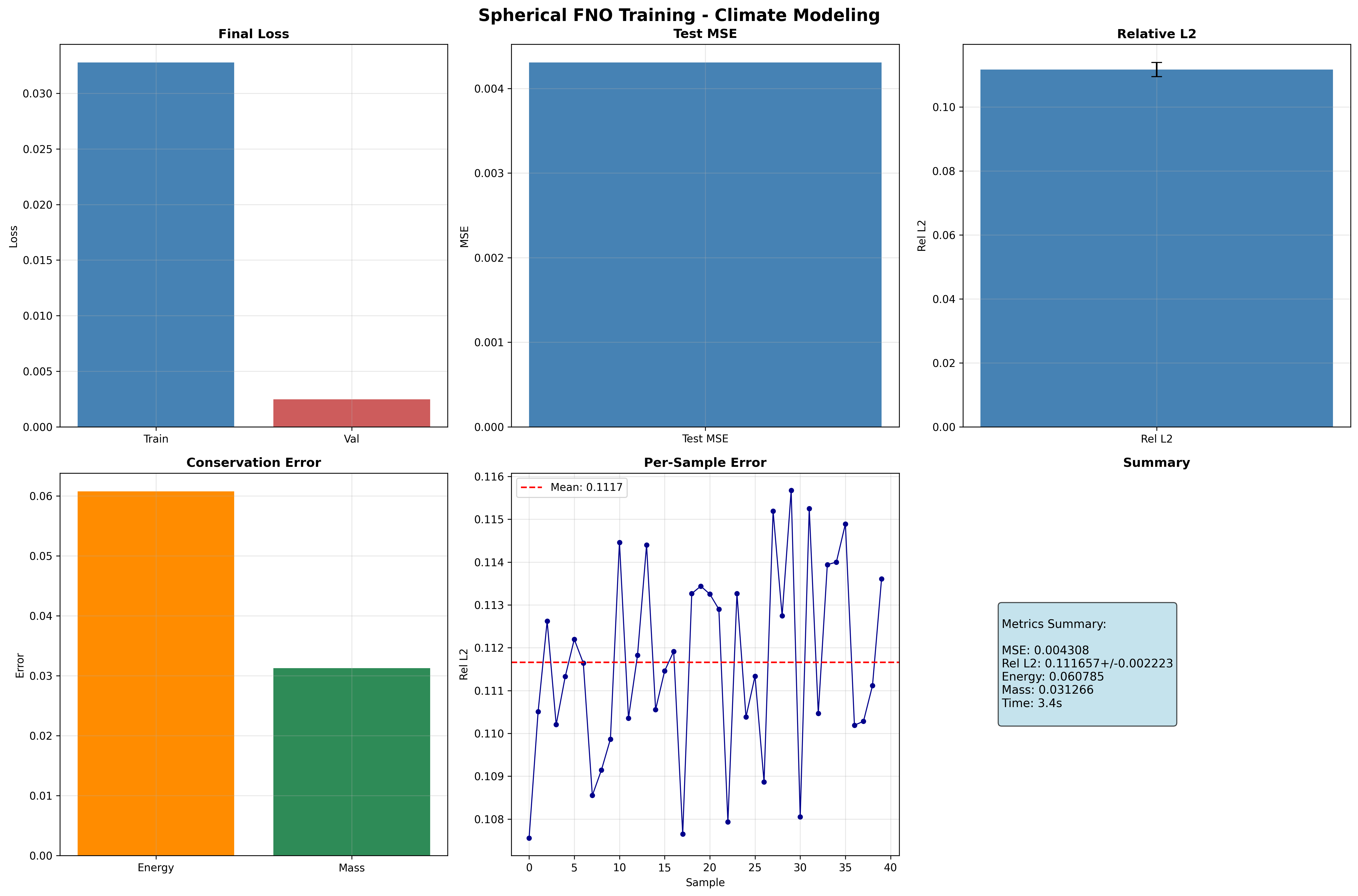
Training Curves

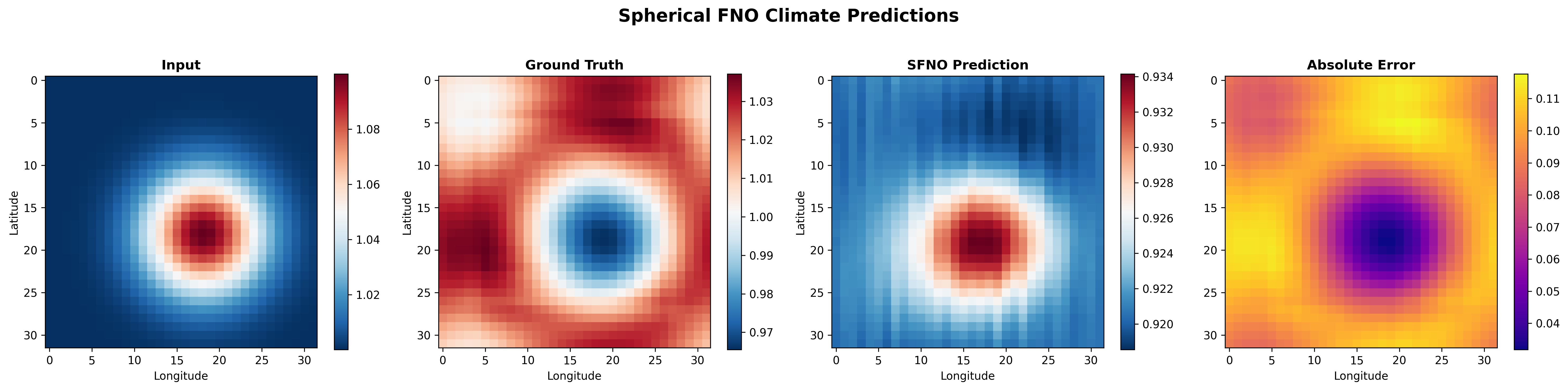
Spherical Predictions

Compare input, ground truth, SFNO prediction, and absolute error on the spherical domain:

Spectral Analysis

Spherical harmonic spectral analysis compares the power spectra of predictions and ground truth:

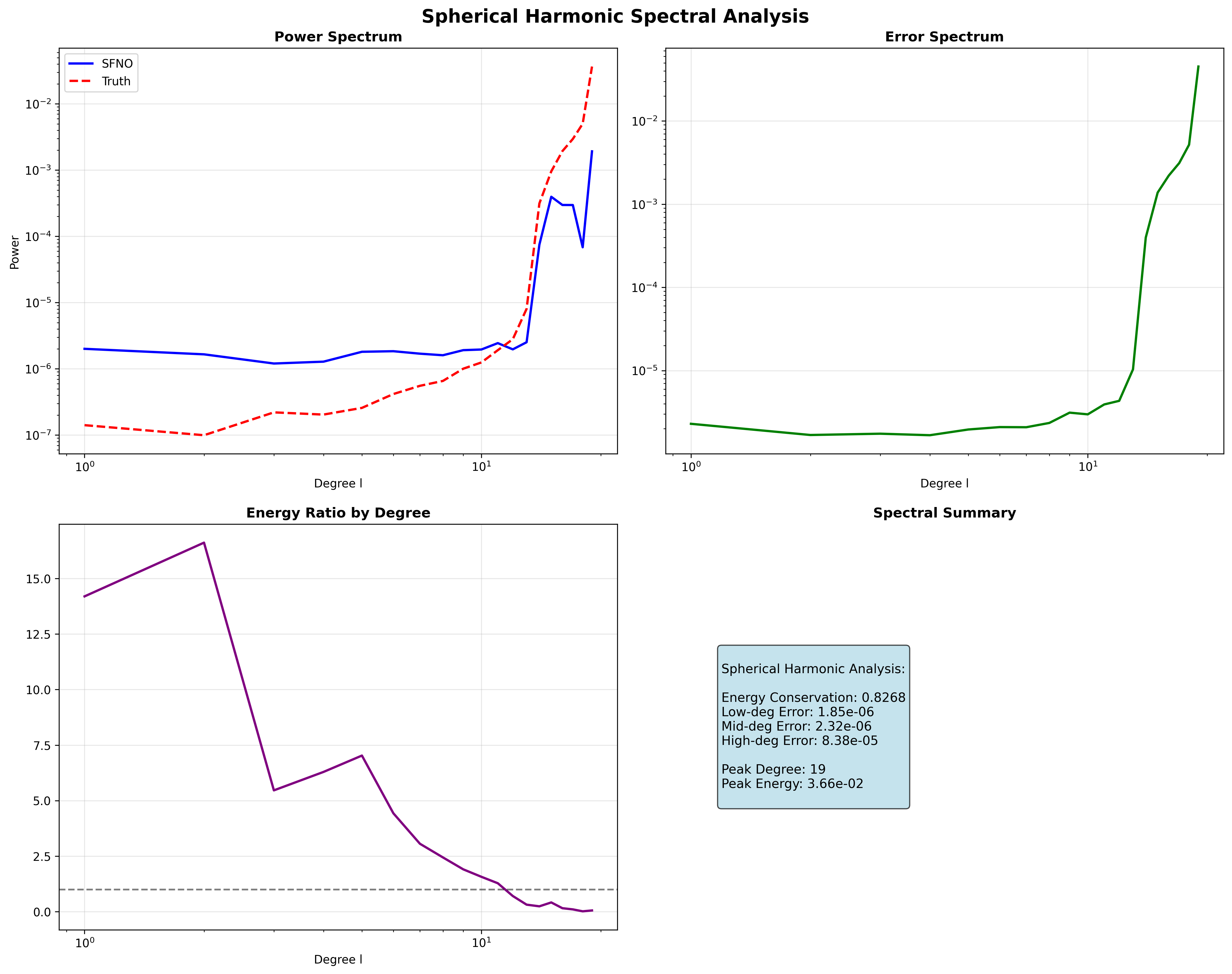
The spectral analysis reveals how well the SFNO captures energy at different spherical harmonic degrees. Low-degree modes (large-scale patterns) are typically captured more accurately than high-degree modes (fine-scale features).

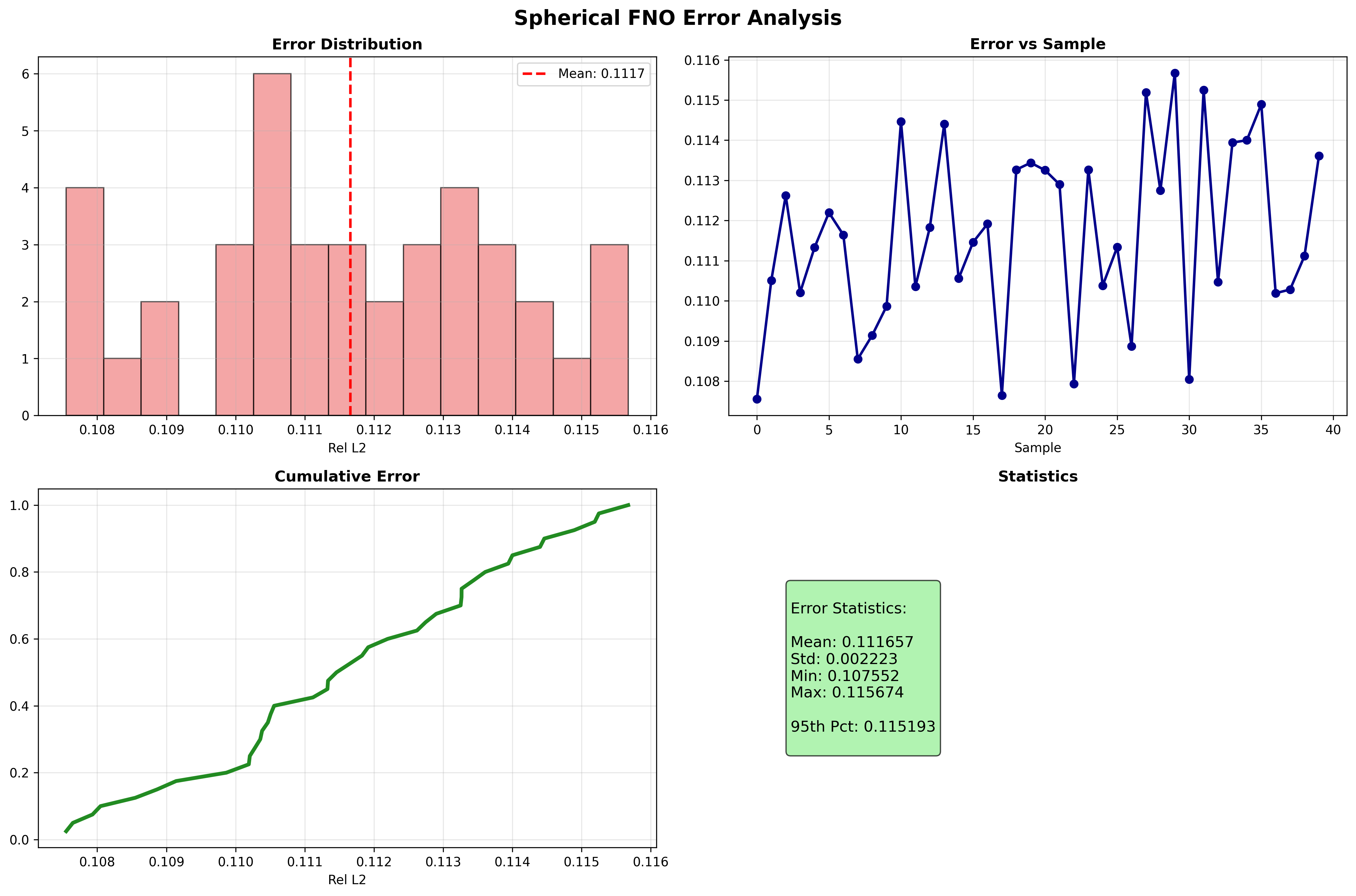
Error Analysis

Terminal Output (visualization generation):

Generating training curves...
Generating spherical predictions...
Generating spectral analysis...
Generating error analysis...

Results Summary

Metric	Value	Notes
Test MSE	0.004308	Mean squared error on test set
Relative L2 Error	0.111657 ± 0.002223	Per-sample mean ± std
Energy Conservation Error	0.060785	Mean absolute energy discrepancy
Mass Conservation Error	0.031266	Mean absolute mass discrepancy
Training Time	3.5s	On single GPU (CudaDevice)
Final Training Loss	0.0328	After 5 epochs
Final Validation Loss	0.0025	After 5 epochs

What We Achieved

• Trained an SFNO for shallow water equation climate data with conservation-aware loss
• Demonstrated energy and mass conservation monitoring through ConservationConfig
• Performed spherical harmonic spectral analysis to evaluate spectral fidelity
• Generated full visualizations of predictions, errors, and spectral properties

Interpretation

The SFNO with only 5 epochs of training achieves a relative L2 error of ~0.112. The conservation metrics show that the model maintains reasonable energy and mass fidelity. The spectral analysis shows that low-degree spherical harmonic modes (large-scale climate patterns) are captured well, while higher-degree modes require additional training. Increasing NUM_EPOCHS, lmax, and RESOLUTION will improve accuracy and conservation properties.

Terminal Output (final summary):

======================================================================
Full SFNO Climate example completed in 3.5s
Mean Relative L2 Error: 0.111657
Results saved to: docs/assets/examples/sfno_climate_comprehensive
======================================================================

Next Steps

Experiments to Try

1. Increase lmax: Try lmax=16 or lmax=32 to capture higher-frequency spherical harmonic modes and improve fine-scale predictions
2. More training epochs: Increase NUM_EPOCHS to 50-100 for better convergence and lower relative L2 error
3. Stronger conservation weighting: Adjust ConservationConfig parameters to more aggressively enforce energy and mass conservation
4. Higher resolution: Increase RESOLUTION to 64 or 128 for higher-fidelity climate field representations
5. Real climate data: Replace synthetic shallow water data with ERA5 reanalysis for realistic weather prediction

Related Examples

Example	Level	What You'll Learn
Simple SFNO Climate	Beginner	Quick-start SFNO on spherical domain
FNO Darcy Tutorial	Intermediate	Full FNO training pipeline for Darcy flow
UNO Darcy Framework	Intermediate	Multi-resolution neural operator architecture
U-FNO Turbulence	Advanced	U-Net enhanced FNO for turbulence modeling
Neural Operator Benchmark	Advanced	Cross-architecture performance comparison

API Reference

• create_climate_sfno - SFNO factory function for climate applications
• ConservationConfig - Conservation law configuration for physics-aware training
• Trainer - Training orchestration with conservation support
• TrainingConfig - Training hyperparameter configuration
• create_shallow_water_loader - Grain-based shallow water equation data loader

Troubleshooting

OOM during training with high lmax

Symptom: jaxlib.xla_extension.XlaRuntimeError: RESOURCE_EXHAUSTED

Cause: Spherical harmonic transforms with high lmax require significant memory, especially at high resolution.

Solution: Reduce lmax, RESOLUTION, or BATCH_SIZE:

# Reduce spectral resolution
LMAX = 8        # Was 32
RESOLUTION = 32  # Was 128
BATCH_SIZE = 4   # Was 16

Alternatively, enable gradient checkpointing:

config = TrainingConfig(gradient_checkpointing=True, gradient_checkpoint_policy="dots_saveable")

NaN in training loss

Symptom: Loss becomes nan after a few epochs.

Cause: Learning rate too high or numerical instability in spherical harmonic transforms.

Solution: Reduce learning rate and add gradient clipping:

import optax

optimizer = optax.chain(
    optax.clip_by_global_norm(1.0),
    optax.adam(1e-4),  # Reduced from 1e-3
)

Conservation loss not decreasing

Symptom: Energy and mass conservation errors remain high despite training.

Cause: Conservation loss weight may be too low relative to the data loss, or the model capacity is insufficient.

Solution: Increase conservation emphasis or model capacity:

# Stronger conservation enforcement
config = TrainingConfig(
    conservation_config=ConservationConfig(
        laws=["energy", "mass"],
        energy_tolerance=1e-8,  # Tighter tolerance
        energy_monitoring=True,
    ))

# Or increase model capacity
model = create_climate_sfno(
    in_channels=3, out_channels=3,
    lmax=16,  # More spectral modes
    rngs=nnx.Rngs(42))

Slow data loading

Symptom: Data loading via Grain takes unexpectedly long.

Cause: Worker count misconfigured or system I/O bottleneck.

Solution: Adjust worker_count based on available CPU cores:

train_loader = create_shallow_water_loader(
    n_samples=200, batch_size=8, resolution=32,
    shuffle=True, seed=42, worker_count=4)  # Use multiple workers