DeepONet on Darcy Flow

Metadata	Value
Level	Intermediate
Runtime	~2 min (CPU) / ~30s (GPU)
Prerequisites	JAX, Flax NNX, Neural Operators basics
Format	Python + Jupyter
Memory	~1 GB RAM

Overview

Train a Deep Operator Network (DeepONet) to learn the Darcy flow operator, which maps permeability coefficient fields to pressure solutions. Unlike FNO which operates on grids, DeepONet uses a branch-trunk architecture that is resolution-independent -- once trained, it can be queried at arbitrary spatial locations.

What You'll Learn

1. Reshape grid data into DeepONet's branch/trunk format
2. Create a DeepONet with branch and trunk networks
3. Train with a custom loop using nnx.Optimizer
4. Evaluate predictions and analyze learned representations

Coming from NeuralOperator (PyTorch)?

If you are familiar with the neuraloperator library's DeepONet implementation:

NeuralOperator (PyTorch)	Opifex (JAX)
DeepONet(branch_net, trunk_net)	DeepONet(branch_sizes, trunk_sizes, rngs=...)
model(u, y)	model(branch_input, trunk_input)
torch.optim.Adam	nnx.Optimizer(model, optax.adam(lr), wrt=nnx.Param)
Manual loss.backward()	nnx.value_and_grad(loss_fn)(model)

Key differences:

1. Flax NNX modules: Explicit PRNG, functional transforms
2. XLA compilation: Use @nnx.jit instead of torch.compile
3. Integrated layer sizes: Pass [input, hidden..., output] lists directly
4. Training options: Custom loop with nnx.Optimizer, or wrap with DeepONetTrainerAdapter for BasicTrainer compatibility

Files

• Python Script: examples/neural-operators/deeponet_darcy.py
• Jupyter Notebook: examples/neural-operators/deeponet_darcy.ipynb

Quick Start

Run the Python Script

source activate.sh && python examples/neural-operators/deeponet_darcy.py

Run the Jupyter Notebook

jupyter lab examples/neural-operators/deeponet_darcy.ipynb

Core Concepts

DeepONet Architecture

DeepONet learns nonlinear operators \(G: u \to G(u)\) mapping between function spaces:

\[G(u)(y) = \sum_{k=1}^{p} b_k(u(x_1), \ldots, u(x_m)) \cdot t_k(y)\]

where:

• Branch network \(b_k\): Encodes the input function \(u\) evaluated at \(m\) sensor locations
• Trunk network \(t_k\): Encodes the evaluation location \(y\)
• Output: Dot product of \(p\)-dimensional branch and trunk embeddings

graph LR
    subgraph Input
        A["Permeability Field<br/>u(x) : (1024,)"]
    end

    subgraph DeepONet["Deep Operator Network"]
        B["Branch Net<br/>MLP: 1024→256→128→64"]
        C["Trunk Net<br/>MLP: 2→128→128→64"]
        D["Dot Product<br/>Σ bₖ · tₖ"]
    end

    subgraph Output
        E["Pressure Field<br/>G(u)(y) : (1024,)"]
    end

    A --> B
    F["Query Locations<br/>y : (1024, 2)"] --> C
    B --> D
    C --> D
    D --> E

    style A fill:#e3f2fd,stroke:#1976d2
    style E fill:#c8e6c9,stroke:#388e3c

FNO vs DeepONet

Aspect	FNO	DeepONet
Grid structure	Fixed resolution required	Arbitrary point evaluation
Data efficiency	Better for grid problems	Requires more data typically
Resolution	Tied to training resolution	Resolution-independent
Architecture	Spectral convolutions	Branch-trunk MLP decomposition

Implementation

Step 1: Imports and Setup

import jax
import jax.numpy as jnp
import numpy as np
from flax import nnx
import optax

from opifex.data.loaders import create_darcy_loader
from opifex.neural.operators.deeponet import DeepONet

Terminal Output:

======================================================================
Opifex Example: DeepONet on Darcy Flow
======================================================================
JAX backend: gpu
JAX devices: [CudaDevice(id=0)]
Resolution: 32x32
Training samples: 200, Test samples: 50
Sensors: 1024, Latent dim: 64

Step 2: Data Preparation

DeepONet requires reshaping grid data into sensor values and coordinate queries:

train_loader = create_darcy_loader(
    n_samples=200, batch_size=200, resolution=32,
    shuffle=True, seed=42, worker_count=0,
)
train_batch = next(iter(train_loader))

# Flatten grid to sensor values for branch input
X_train_branch = X_train_grid.reshape(N, -1)  # (200, 1024)

# Create coordinate grid for trunk input
x_coords = np.linspace(0, 1, 32)
y_coords = np.linspace(0, 1, 32)
xx, yy = np.meshgrid(x_coords, y_coords)
trunk_coords = np.stack([xx.ravel(), yy.ravel()], axis=-1)  # (1024, 2)

Terminal Output:

Branch input: (200, 1024)
Trunk input:  (1024, 2)
Target:       (200, 1024)

Step 3: Model Creation

The branch and trunk must have matching output dimensions (latent_dim=64):

model = DeepONet(
    branch_sizes=[1024, 256, 128, 64],  # sensors → latent
    trunk_sizes=[2, 128, 128, 64],       # coords → latent
    activation="gelu",
    rngs=nnx.Rngs(42),
)

Terminal Output:

Model: DeepONet (latent_dim=64)
Branch: [1024, 256, 128, 64]
Trunk:  [2, 128, 128, 64]
Total parameters: 328,704

Step 4: Training with Custom Loop

DeepONet takes separate branch and trunk inputs, so we use nnx.Optimizer directly instead of the grid-based Trainer:

opt = nnx.Optimizer(model, optax.adam(1e-3), wrt=nnx.Param)

@nnx.jit
def train_step(model, opt, x_branch, y_target):
    def loss_fn(model):
        trunk_batch = jnp.broadcast_to(trunk_jax[None], (batch_size, *trunk_jax.shape))
        y_pred = model(x_branch, trunk_batch)
        return jnp.mean((y_pred - y_target) ** 2)

    loss, grads = nnx.value_and_grad(loss_fn)(model)
    opt.update(model, grads)
    return loss

Terminal Output:

Optimizer: Adam (lr=0.001)

Starting training (30 epochs)...
  Epoch   1/30: train_loss=0.040347, val_loss=0.003253
  Epoch  10/30: train_loss=0.000027, val_loss=0.000026
  Epoch  20/30: train_loss=0.000014, val_loss=0.000013
  Epoch  30/30: train_loss=0.000010, val_loss=0.000010

Training completed in 2.4s
Final train loss: 9.870162e-06
Final val loss:   9.561398e-06

Step 5: Evaluation

Terminal Output:

Running evaluation...
Test MSE:         0.000010
Test Relative L2: 0.320663
Min Relative L2:  0.230521
Max Relative L2:  0.503679

======================================================================
DeepONet Darcy Flow example completed in 2.4s
Test MSE: 0.000010, Relative L2: 0.320663
Results saved to: docs/assets/examples/deeponet_darcy
======================================================================

Visualization

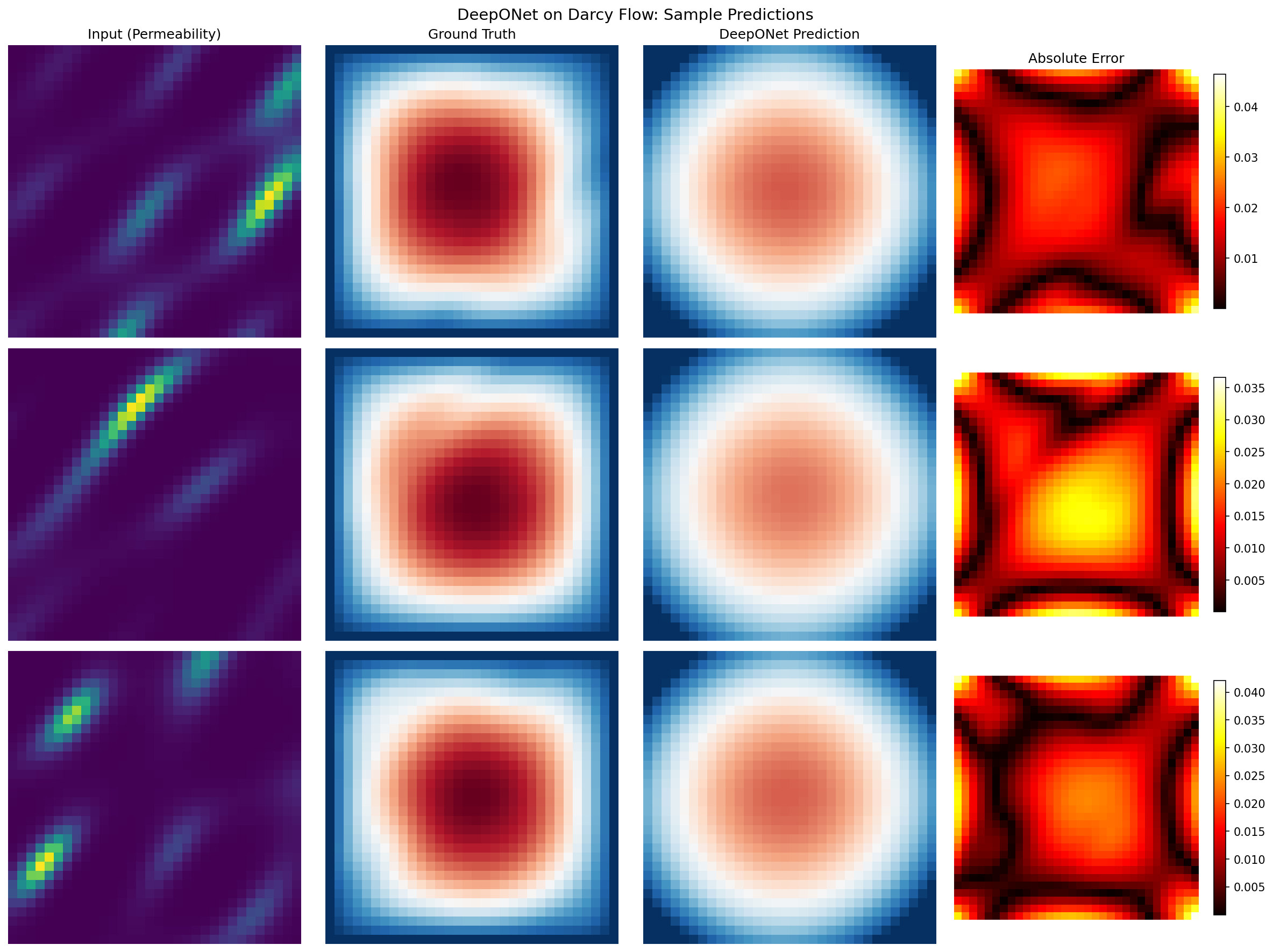
Sample Predictions

Input permeability, ground truth pressure, DeepONet prediction, and absolute error for three test samples:

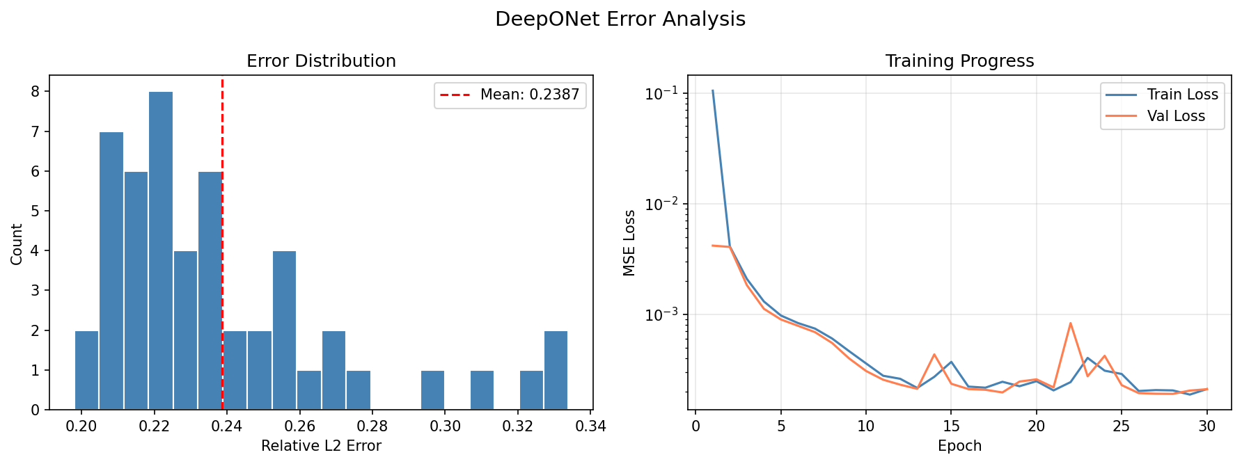
Error Analysis

Error distribution across test samples and training convergence:

Branch-Trunk Embeddings

The learned branch and trunk representations reveal how DeepONet decomposes the operator:

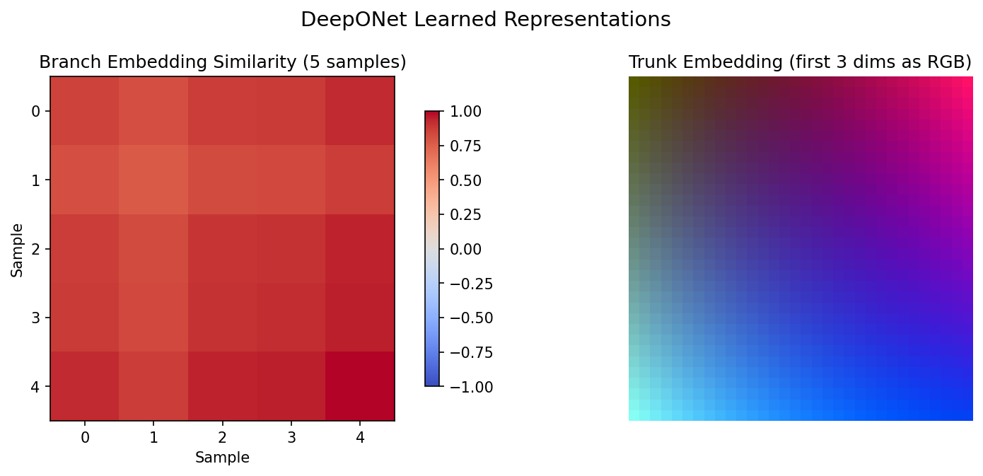
The trunk embedding (right) shows the spatial structure learned by the trunk network, while the branch similarity matrix (left) shows how different input functions are encoded in the latent space.

Results Summary

Metric	Value
Test MSE	0.000010
Relative L2 Error	0.321
Training Time	2.4s (GPU)
Parameters	328,704
Final Train Loss	9.87e-6
Final Val Loss	9.56e-6

Next Steps

Experiments to Try

1. Increase latent dimension: Try latent_dim=128 for more expressive embeddings
2. Add more hidden layers: Deeper branch/trunk networks for complex operators
3. Higher resolution: Apply to 64x64 or 128x128 grids (adjust sensor count)
4. Periodic BCs: Modify trunk network to handle periodic boundary conditions

Related Examples

Example	Level	What You'll Learn
DeepONet on Antiderivative	Intermediate	Classic operator learning task
FNO on Darcy Flow	Intermediate	Compare with grid-based FNO
UNO on Darcy Flow	Intermediate	Multi-scale UNO approach

API Reference

• DeepONet - Deep Operator Network model class
• DeepONetTrainerAdapter - Wraps DeepONet for BasicTrainer compatibility (accepts {'branch': ..., 'trunk': ...} dict input)
• create_darcy_loader - Darcy flow data loader

Troubleshooting

Shape mismatch between branch and trunk outputs

Symptom: Error like Incompatible shapes for dot: got (batch, 64) and (batch, 128).

Cause: Branch and trunk networks have different final dimensions.

Solution: Ensure the last element of branch_sizes and trunk_sizes match:

model = DeepONet(
    branch_sizes=[1024, 256, 128, 64],  # Last: 64
    trunk_sizes=[2, 128, 128, 64],       # Last: 64 (must match!)
    rngs=nnx.Rngs(42),
)

DeepONet doesn't work with Trainer

Symptom: Trainer.fit() fails with DeepONet.

Cause: Trainer expects single-input models, but DeepONet takes two inputs.

Solution: Use a custom training loop with nnx.Optimizer:

opt = nnx.Optimizer(model, optax.adam(1e-3), wrt=nnx.Param)

@nnx.jit
def train_step(model, opt, x_branch, x_trunk, y_target):
    def loss_fn(model):
        y_pred = model(x_branch, x_trunk)
        return jnp.mean((y_pred - y_target) ** 2)

    loss, grads = nnx.value_and_grad(loss_fn)(model)
    opt.update(model, grads)
    return loss

High relative L2 error

Symptom: Relative L2 error > 0.5 even after convergence.

Cause: DeepONet requires more data than FNO for grid problems. The branch network needs to learn to encode the full input function from sensor values.

Solution: Increase training data or sensor count:

# More training samples
train_loader = create_darcy_loader(n_samples=500, ...)

# Or higher sensor resolution (64x64 = 4096 sensors)
branch_sizes = [4096, 512, 256, 64]