Darcy Flow Dataset Analysis
| Metadata | Value |
|---|---|
| Level | Intermediate |
| Runtime | ~2 min (CPU) |
| Prerequisites | JAX, NumPy, Darcy Flow basics |
| Format | Python + Jupyter |
Overview
Darcy flow describes fluid flow through porous media, governed by the elliptic PDE: \(-\nabla \cdot (k(x) \nabla u(x)) = f(x)\), where \(k\) is the permeability field and \(u\) is the pressure field. This example provides full analysis of Darcy flow datasets generated by the Opifex framework, including field statistics, spatial gradient analysis, resolution scaling, and data quality metrics.
Understanding dataset properties is essential before training neural operators — field statistics reveal normalization requirements, gradient analysis validates physical consistency, and resolution scaling guides computational budget allocation.
What You'll Learn
- Generate Darcy flow datasets with
generate_darcyat multiple resolutions - Analyze field statistics (mean, std, dynamic range) for permeability and pressure
- Compute spatial gradient correlations between input and output fields
- Evaluate resolution scaling performance (samples/second, time scaling)
- Visualize resolution-dependent statistics and performance metrics
Coming from neuraloperator (PyTorch)?
| neuraloperator (PyTorch) | Opifex (JAX) |
|---|---|
torch.utils.data.DataLoader(dataset) |
generate_darcy(n_samples=, resolution=, seed=) |
Manual torch.meshgrid for coordinates |
GridEmbedding2D(in_channels=, grid_boundaries=) |
torch.gradient() (limited) |
jnp.gradient(field, axis=) (NumPy-compatible) |
| Manual per-sample loop | Single vmapped on-device batch |
Key difference: Opifex generates the whole batch on-device in one call. generate_darcy
is a vmapped generator that returns a {"input": (n, 1, H, W), "output": (n, 1, H, W)}
dictionary for a given resolution and seed, which is then split into a per-sample list for
analysis. No external data-loading framework is required — generation runs on the JAX
device and is fully reproducible from the seed.
Files
- Python Script:
examples/data/darcy_flow_analysis.py - Jupyter Notebook:
examples/data/darcy_flow_analysis.ipynb
Quick Start
Core Concepts
Darcy Flow as a Benchmark Problem
Darcy flow is the canonical benchmark for neural operators (used in PDEBench and the original FNO paper). The problem maps a permeability field \(k(x)\) to a pressure field \(u(x)\), making it ideal for operator learning since it requires learning a nonlinear mapping between function spaces.
graph LR
    A["Permeability k(x)<br/>(Input Field)"] --> B["Darcy PDE<br/>-div(k grad u) = f"]
    B --> C["Pressure u(x)<br/>(Output Field)"]
    D["generate_darcy<br/>(vmapped on-device)"] --> A
    D --> C

    style A fill:#e3f2fd
    style C fill:#c8e6c9
    style B fill:#fff3e0
Analysis Pipeline
| Analysis Type | What It Measures | Why It Matters |
|---|---|---|
| Field Statistics | Mean, std, min, max, dynamic range | Normalization requirements |
| Spatial Gradients | Gradient magnitudes, input-output correlation | Physical consistency |
| Resolution Scaling | Generation time, samples/sec across resolutions | Computational budget |
| Data Quality | NaN/Inf checks, range validation | Training stability |
Implementation
Step 1: Data Generation with generate_darcy
Generate datasets at multiple resolutions using Opifex's vmapped on-device generator.
generate_darcy returns a {"input", "output"} dictionary of channels-first
(n, 1, H, W) fields, which is split into a per-sample list for analysis:
from opifex.data.sources import generate_darcy

data = generate_darcy(n_samples=100, resolution=64, seed=42)
samples = [
    {"input": data["input"][i], "output": data["output"][i]}
    for i in range(100)
]
Terminal Output:
DARCY FLOW DATASET ANALYSIS
================================================================================

Analyzing resolution: 64x64
  Generated 100 samples in 1.80s
  Rate: 55.5 samples/second

Analyzing resolution: 128x128
  Generated 100 samples in 4.29s
  Rate: 23.3 samples/second
Step 2: Field Statistics Analysis
Compute full statistics for permeability (input) and pressure (output) fields:
stats = _compute_field_statistics(fields)
# Returns: mean, std, min, max, median, q25, q75, dynamic_range, coefficient_of_variation
Terminal Output:
ANALYSIS COMPLETE
================================================================================
Resolution 64x64:
  Generation time: 1.80s
  Samples/second: 55.5
  Input mean: 0.1782
  Output mean: 0.2214
Resolution 128x128:
  Generation time: 4.29s
  Samples/second: 23.3
  Input mean: 0.1780
  Output mean: 0.2254
Step 3: Spatial Gradient Analysis
Analyze spatial gradients to verify physical consistency between permeability and pressure:
spatial_results = _analyze_spatial_patterns(inputs, outputs)
# Computes: gradient magnitudes, input-output correlation, gradient correlation
The gradient analysis verifies that: - High permeability regions correspond to lower pressure gradients (Darcy's law) - Spatial patterns are physically consistent across samples
Step 4: Resolution Scaling
Compare dataset properties and generation performance across resolutions:
comparisons = _compare_resolutions(datasets)
# Returns: resolution_scale, time_scale, efficiency_ratio
Visualization
The analysis generates three plot types:
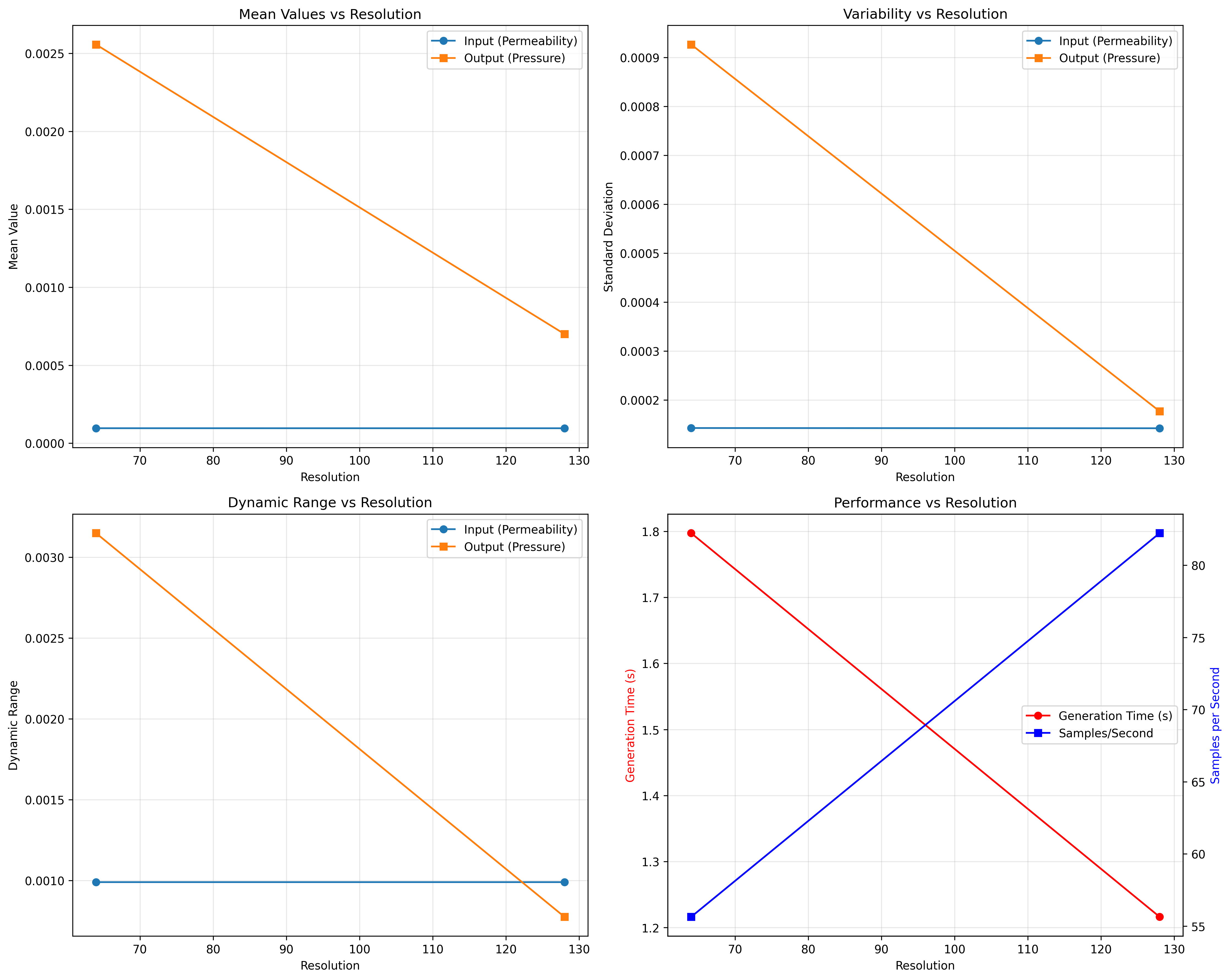
Results Summary
| Metric | 64x64 | 128x128 | Scaling |
|---|---|---|---|
| Generation Time | 1.80s | 4.29s | Quadratic |
| Samples/Second | 55.5 | 23.3 | Inverse quadratic |
| Input Mean | 0.1782 | 0.1780 | Resolution-invariant |
| Output Mean | 0.2214 | 0.2254 | Resolution-invariant |
Key Takeaways
- Generation time scales quadratically with resolution (expected for 2D fields)
- Field statistics remain consistent across resolutions (good for multi-resolution training)
- Spatial gradient correlations validate physical consistency of generated data
- The vmapped
generate_darcygenerates the whole batch on-device and is fully reproducible from the seed
Next Steps
Experiments to Try
- Higher resolutions: Test 256x256 and 512x512 to observe scaling behavior
- Viscosity sweep: Vary
viscosity_rangeto see how it affects field statistics - Larger datasets: Generate 1000+ samples and track generation throughput
Related Examples
| Example | Level | What You'll Learn |
|---|---|---|
| Spectral Analysis (Darcy) | Advanced | Frequency domain analysis of these datasets |
| FNO Darcy Full | Intermediate | Train FNO on Darcy flow data |
| Neural Operator Benchmark | Advanced | Cross-architecture comparison on Darcy flow |
API Reference
generate_darcy- Vmapped on-device Darcy flow data generatorGridEmbedding2D- Spatial coordinate embedding for grid data
Troubleshooting
generate_darcy returns constant fields
Symptom: All samples have identical permeability or pressure fields.
Cause: The generator is vmapped over a per-sample key derived from the seed; a constant batch usually indicates the resolution or sample count was misconfigured.
Solution: Vary the seed to produce a different deterministic batch, and confirm
n_samples > 1. Each sample in the returned (n, 1, H, W) arrays is distinct.
Slow generation at high resolutions
Symptom: 256x256 or higher takes very long to generate.
Cause: Generation time scales quadratically with resolution.
Solution: Generate a smaller number of high-resolution samples:
NaN values in gradient analysis
Symptom: _analyze_spatial_patterns returns NaN for correlation.
Cause: Constant fields produce zero variance, making correlation undefined.
Solution: Check field statistics first. If std is near zero, the field
is effectively constant and gradient analysis is not meaningful.