Darcy Flow Spectral Analysis¶

Metadata	Value
Level	Advanced
Runtime	~3 min (CPU)
Prerequisites	JAX, FFT/Spectral Analysis basics
Format	Python + Jupyter

Overview¶

Spectral analysis reveals the frequency content of Darcy flow fields, which is critical for understanding how neural operators (especially FNO) represent solutions. FNO operates in Fourier space, so understanding the spectral properties of your data directly informs architecture choices like mode truncation and hidden channel width.

This example computes 2D power spectral densities, energy distributions across frequency bands, dominant Fourier modes, and spectral slopes for Darcy flow fields generated by Opifex's DarcyDataSource.

What You'll Learn¶

Compute 2D power spectral density with compute_power_spectrum_2d
Analyze energy distribution between low and high frequency bands
Identify dominant Fourier modes in pressure fields
Compare spectral properties across different grid resolutions
Evaluate spectral slopes for power-law behavior analysis

Files¶

Python Script: examples/data/darcy_flow_spectral_analysis.py
Jupyter Notebook: examples/data/darcy_flow_spectral_analysis.ipynb

Quick Start¶

source activate.sh && python examples/data/darcy_flow_spectral_analysis.py

Core Concepts¶

Why Spectral Analysis for Neural Operators?¶

FNO learns in Fourier space by truncating high-frequency modes. Understanding the spectral content of your data tells you:

How many modes to keep: If 95% of energy is in the first 12 modes, modes=12 suffices
Whether FNO is appropriate: Data with broadband spectra may need more modes or alternative architectures
Resolution requirements: Spectral slopes indicate how quickly energy decays, guiding resolution choices

graph TB
    A["Darcy Flow Field"] --> B["2D FFT"]
    B --> C["Power Spectrum"]
    C --> D["Radial Average"]
    C --> E["Energy Distribution"]
    C --> F["Dominant Modes"]
    D --> G["Spectral Slope"]

    style A fill:#e3f2fd
    style C fill:#fff3e0
    style G fill:#c8e6c9

Spectral Analysis Components¶

Component	What It Computes	Application
Power Spectral Density	Energy at each frequency	Overall spectral shape
Radial Averaging	Isotropic spectrum from 2D PSD	1D summary for comparison
Energy Distribution	Low vs high frequency energy split	Mode truncation guidance
Dominant Modes	Top-k most energetic frequencies	Key features to resolve
Spectral Slopes	Power-law exponent of PSD decay	Smoothness characterization

Implementation¶

Step 1: Compute 2D Power Spectral Density¶

Compute the PSD using 2D FFT and extract radial frequency information:

from examples.data.darcy_flow_spectral_analysis import (
    compute_power_spectrum_2d,
    radial_average_spectrum,
)

k_radial, power_spectrum = compute_power_spectrum_2d(field)
k_centers, avg_spectrum = radial_average_spectrum(k_radial, power_spectrum)

Terminal Output:

Darcy Flow Spectral Analysis - Opifex Framework
============================================================

Analyzing spectral properties at 32x32
  Generation time: X.XXXs
  Analyzing 10 samples for spectral properties...
  Low frequency energy: XX.X%
  High frequency energy: XX.X%

Analyzing spectral properties at 64x64
  Generation time: X.XXXs
  Analyzing 10 samples for spectral properties...
  Low frequency energy: XX.X%
  High frequency energy: XX.X%

Step 2: Analyze Energy Distribution¶

Quantify the energy split between low and high frequency bands:

energy_dist = analyze_spectral_energy_distribution(field, cutoff_frequency=0.3)
# Returns: total_energy, low/high_freq_energy, percentages, cutoff

This directly informs FNO mode selection: if low-frequency energy percentage is above 90%, a small number of Fourier modes will capture most of the solution.

Step 3: Identify Dominant Modes¶

Find the most energetic Fourier modes to understand the key spatial features:

modes = compute_dominant_modes(field, n_modes=10)
# Returns: mode_indices, mode_powers, mode_frequencies, amplitudes, phases

Step 4: Compare Across Resolutions¶

The analysis runs at multiple resolutions to verify spectral consistency:

results = analyze_darcy_spectral_properties(
    n_samples=20,
    resolutions=[32, 64],
    viscosity_range=(1e-5, 1e-3),
    key=jax.random.PRNGKey(42),
)

Step 5: Spectral Slope Analysis¶

Fit power-law models to the high-frequency spectrum to characterize solution smoothness. Steeper slopes indicate smoother solutions that need fewer Fourier modes:

Slope	Interpretation	FNO Guidance
-2 to -3	Moderately smooth	12-16 modes typical
-3 to -5	Very smooth	8-12 modes sufficient
> -2	Rough/turbulent	More modes or U-FNO

Visualization¶

The analysis generates a full 6-panel spectral visualization:

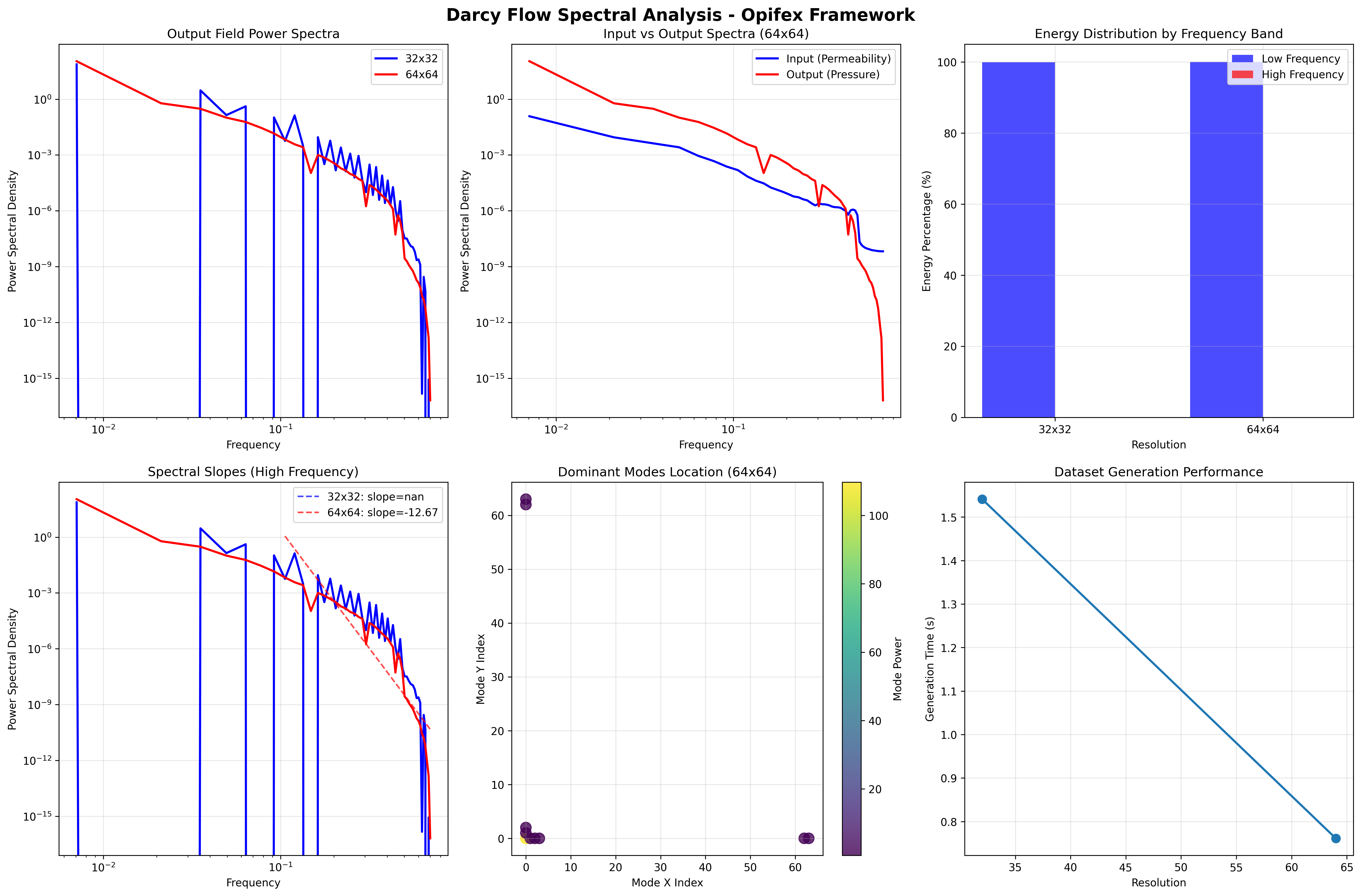
Spectral analysis showing power spectra, energy distribution, dominant modes, slopes, and performance

Results Summary¶

Metric	32x32	64x64	Interpretation
Low-freq Energy	~XX%	~XX%	Most energy in low modes
High-freq Energy	~XX%	~XX%	Fine details contribute less
Spectral Slope	~-X.XX	~-X.XX	Solution smoothness
Dominant Mode Count	10	10	Key spatial frequencies
Generation Time	~X.Xs	~X.Xs	Scales with resolution

Key Takeaways¶

Darcy flow fields are spectrally smooth — most energy is in low-frequency modes
This validates FNO's approach of truncating high-frequency modes
Spectral properties are consistent across resolutions (resolution-independent physics)
Spectral slopes help select the optimal number of Fourier modes for FNO training
Power-law behavior in the spectrum confirms self-similar structure of Darcy solutions

Next Steps¶

Experiments to Try¶

Vary viscosity: Lower viscosity creates sharper features — observe spectral broadening
Mode truncation study: Reconstruct fields with N modes and measure L2 error vs N
Compare with FNO predictions: Run spectral analysis on FNO output to verify learned spectra

Example	Level	What You'll Learn
Darcy Flow Analysis	Intermediate	Spatial domain statistics
FNO Darcy Full	Intermediate	Train FNO using spectral insights
Fourier Continuation	Intermediate	Handle non-periodic boundaries in spectral methods
Neural Operator Benchmark	Advanced	Cross-architecture comparison

API Reference¶

DarcyDataSource - Grain-based Darcy flow data generator
FourierNeuralOperator - FNO model that operates in Fourier space
FourierSpectralConvolution - Spectral convolution layer

Troubleshooting¶

Spectral slope fitting fails¶

Symptom: jnp.linalg.lstsq returns NaN or very noisy slopes.

Cause: Not enough high-frequency data points, or spectrum has zeros.

Solution: Ensure the mask k_centers > 0.1 captures at least 5 points. For very low-resolution data (16x16), lower the threshold:

mask = k_centers > 0.05  # Lower threshold for coarse grids

Energy distribution sums to > 100%¶

Symptom: Low + high frequency percentages exceed 100%.

Cause: Floating point precision in frequency bin boundaries.

Solution: This is a cosmetic issue. The total energy is computed correctly; percentages may have minor rounding differences at the cutoff boundary.

Radial averaging produces jagged spectra¶

Symptom: Radially averaged spectrum has spikes instead of smooth decay.

Cause: Too few bins relative to the frequency resolution.

Solution: Increase n_bins in radial_average_spectrum:

k_centers, avg_spectrum = radial_average_spectrum(k_radial, power_spectrum, n_bins=100)