PINO on Burgers Equation¶

Metadata	Value
Level	Advanced
Runtime	~3 min (CPU) / ~1-2 min (GPU)
Prerequisites	JAX, Flax NNX, FNO, PDEs basics
Format	Python + Jupyter
Memory	~2 GB RAM

Overview¶

This tutorial trains a Physics-Informed Neural Operator (PINO) on the 1D viscous Burgers equation. PINO pairs the FNO architecture with a physics-informed loss so the learned operator both fits the data and satisfies the governing PDE.

The Burgers equation:

\[\frac{\partial u}{\partial t} + u \frac{\partial u}{\partial x} = \nu \frac{\partial^2 u}{\partial x^2}\]

where \(u\) is velocity, \(\nu\) is viscosity, and subscripts denote partial derivatives. The spatial domain is the periodic interval \([0, 1)\).

The genuine PINO setup¶

Following Li et al. (2021), Physics-Informed Neural Operator for Learning Partial Differential Equations, and the reference implementation in neuraloperator (scripts/train_burgers_pino.py), the operator maps the initial condition \(u(x, 0)\) — broadcast/repeated across the time axis — to the full space-time solution \(u(t, x)\), a 2D field over \((\text{time}, \text{space})\).

A 2D FNO is the backbone: the input is the tiled initial condition of shape (batch, 1, nt, nx) and the output is the predicted field (batch, 1, nt, nx).

Training minimises three terms (cf. neuralop.losses.equation_losses BurgersEqnLoss + ICLoss):

data loss: mean relative L2 between the predicted and the ground-truth space-time trajectory,
IC loss: MSE between the predicted \(t = 0\) slice and the true initial condition,
equation loss: the mean-squared Burgers PDE residual \(u_t + u\,u_x - \nu\,u_{xx}\) evaluated by finite differences over the whole predicted field.

The viscosity \(\nu = 0.01\) is shared between the data-generating spectral solver and the equation loss, so the supervised physics is self-consistent.

What You'll Learn¶

Understand the PINO operator: IC tiled over time \(\to\) full \(u(t, x)\) field
Implement the Burgers PDE residual with finite differences
Combine data + IC + equation losses with fixed weights
Generate self-consistent Burgers trajectories with the spectral solver

Coming from NeuralOperator (PyTorch)?¶

If you are familiar with the neuraloperator library's PINO example:

NeuralOperator (PyTorch)	Opifex (JAX)
`FNO(n_modes=(16,16), ...)` (2D)	`FourierNeuralOperator(spatial_dims=2, ...)`
`BurgersEqnLoss(visc=0.01, method="fdm")`	`equation_loss()` finite-difference residual
`ICLoss()`	MSE on the predicted `pred[:, 0, :]` slice
`LpLoss(d=2, p=2)`	`relative_l2()` over the full trajectory
`Relobralo` adaptive aggregator	Fixed weights (data / IC / equation)
`Burgers1dTimeDataProcessor` (repeat `x`)	`tile_ic()` repeats the IC over the time axis

Key differences:

On-device data generation: trajectories are built with the pseudo-spectral ETDRK4 Burgers solver, vmapped over the batch — no external data files
Fixed loss weights: a clean, reproducible alternative to the reference's Relobralo aggregator; the weights follow the same (data, IC, equation) ordering
JAX transforms: a single jit(vmap(...)) call generates the whole dataset

Files¶

Python Script: examples/neural-operators/pino_burgers.py
Jupyter Notebook: examples/neural-operators/pino_burgers.ipynb

Quick Start¶

Run the Python Script¶

source activate.sh && python examples/neural-operators/pino_burgers.py

Run the Jupyter Notebook¶

jupyter lab examples/neural-operators/pino_burgers.ipynb

Core Concepts¶

Physics-Informed Loss¶

The total loss combines three components:

\[\mathcal{L}_{\text{total}} = w_d\,\mathcal{L}_{\text{data}} + w_{ic}\,\mathcal{L}_{\text{IC}} + w_{eq}\,\mathcal{L}_{\text{eqn}}\]

with fixed weights \(w_d = 1.0\), \(w_{ic} = 5.0\), \(w_{eq} = 0.5\), where

\[\mathcal{L}_{\text{data}} = \mathbb{E}\left[\frac{\lVert \hat u - u \rVert_2}{\lVert u \rVert_2}\right], \qquad \mathcal{L}_{\text{IC}} = \mathbb{E}\left[\big(\hat u(0, \cdot) - u(0, \cdot)\big)^2\right]\]

and the equation loss is the mean-squared Burgers PDE residual over the full predicted field:

\[\mathcal{L}_{\text{eqn}} = \mathbb{E}\left[\left(u_t + u\,u_x - \nu\,u_{xx}\right)^2\right]\]

PINO Architecture¶

graph LR
    subgraph Input
        A["Initial Condition<br/>u(x,0) tiled over time<br/>R^(1×11×128)"]
    end

    subgraph PINO["Physics-Informed Neural Operator"]
        B["2D FNO Backbone<br/>(4 spectral layers)"]
        C["Data Loss<br/>relative L2 vs u(t,x)"]
        D["IC Loss<br/>MSE on t=0 slice"]
        E["Equation Loss<br/>Burgers PDE residual"]
    end

    subgraph Output
        F["Space-Time Solution<br/>u(t,x) : R^(1×11×128)"]
    end

    A --> B --> F
    F --> C
    F --> D
    F --> E
    C --> G["Total Loss"]
    D --> G
    E --> G

    style A fill:#e3f2fd,stroke:#1976d2
    style F fill:#c8e6c9,stroke:#388e3c
    style G fill:#fff3e0,stroke:#f57c00

Implementation¶

Step 1: Imports and Setup¶

import jax
import jax.numpy as jnp
from flax import nnx

from opifex.neural.operators.fno.base import FourierNeuralOperator
from opifex.physics.spectral.steppers import solve_burgers_spectral

Terminal Output:

======================================================================
Opifex Example: PINO on 1D Burgers Equation
======================================================================
JAX backend: gpu
JAX devices: [CudaDevice(id=0)]
Grid: nx=128, nt=11, viscosity=0.01
Trajectories: train=1000, test=200
FNO config: modes=16, width=32, layers=4
Loss weights: data=1.0, ic=5.0, equation=0.5
Spacings: dx=0.00781, dt=0.10000

Step 2: Data Generation¶

Initial conditions are periodic spectral Gaussian random fields (the canonical FNO/PINO benchmark IC, covariance \(\sigma^2(-\Delta + \tau^2 I)^{-\gamma}\)). Each IC is evolved to the full trajectory \(u(t, x)\) with the pseudo-spectral ETDRK4 Burgers solver, vmapped over the batch on device. solve_burgers_spectral returns (num_snapshots + 1, nx) real snapshots including the initial condition, i.e. exactly the nt = NUM_TIME time frames the model trains on.

def per_sample(key):
    ic = _burgers_ic(key, NUM_SPACE)
    return solve_burgers_spectral(
        ic, VISCOSITY, domain_extent=1.0, time_final=1.0,
        num_steps=250, num_snapshots=NUM_TIME - 1,
    )

keys = jax.vmap(jax.random.PRNGKey)(seed + jnp.arange(n_samples))
trajectories = jax.jit(jax.vmap(per_sample))(keys)  # (n, nt, nx)

Terminal Output:

Generating Burgers space-time trajectories (jit+vmap spectral solver)...
Train trajectories: (1000, 11, 128)
Test trajectories:  (200, 11, 128)

Step 3: PDE Residual¶

The residual is computed by finite differences over the predicted field (batch, nt, nx): a forward difference in time, periodic central differences in space. This mirrors neuralop.losses.equation_losses.BurgersEqnLoss (method="fdm").

def compute_burgers_residual(u, dx, dt, nu):
    u_t = (u[:, 1:, :] - u[:, :-1, :]) / dt          # forward diff in time
    u_level = u[:, :-1, :]
    u_right = jnp.roll(u_level, shift=-1, axis=-1)    # periodic wrap
    u_left = jnp.roll(u_level, shift=1, axis=-1)
    u_x = (u_right - u_left) / (2.0 * dx)
    u_xx = (u_right - 2.0 * u_level + u_left) / (dx**2)
    return u_t + u_level * u_x - nu * u_xx

Step 4: Model Creation¶

The IC is tiled over the time axis to shape (batch, 1, nt, nx); a 2D FNO maps it to the full space-time field. Space is periodic, so no domain padding is used.

model = FourierNeuralOperator(
    in_channels=1,
    out_channels=1,
    hidden_channels=32,
    modes=16,
    num_layers=4,
    spatial_dims=2,
    positional_embedding=True,
    domain_padding=0.0,
    rngs=nnx.Rngs(SEED),
)

Terminal Output:

Creating PINO model (2D FNO backbone over (time, space))...
Model parameters: 4,203,009

Step 5: Training¶

AdamW with a cosine-decayed learning rate (decayed over the total number of mini-batch updates). Each step adds the data, IC, and equation losses with fixed weights.

def pino_loss_fn(model, ic_tiled, trajectory, ic):
    pred = model(ic_tiled)[:, 0]                       # (batch, nt, nx)
    data_loss = relative_l2(pred, trajectory)          # data L2
    ic_loss = jnp.mean((pred[:, 0, :] - ic) ** 2)      # IC anchor
    eqn_loss = equation_loss(pred, DX, DT, VISCOSITY)  # PDE residual
    total = data_loss + 5.0 * ic_loss + 0.5 * eqn_loss
    return total, {"data": data_loss, "ic": ic_loss, "equation": eqn_loss}

Terminal Output:

Starting PINO training...
Optimizer: AdamW (cosine-decayed lr from 0.001)
Epoch    1/800: Total=1.388993, Data=0.633944, IC=8.641672e-02, Equation=6.459318e-01
Epoch  100/800: Total=0.089785, Data=0.039767, IC=2.801668e-03, Equation=7.201982e-02
Epoch  200/800: Total=0.086708, Data=0.037631, IC=2.748990e-03, Equation=7.066499e-02
Epoch  300/800: Total=0.085388, Data=0.036472, IC=2.710348e-03, Equation=7.072789e-02
Epoch  400/800: Total=0.084342, Data=0.035752, IC=2.695936e-03, Equation=7.022096e-02
Epoch  500/800: Total=0.084057, Data=0.035349, IC=2.689569e-03, Equation=7.052071e-02
Epoch  600/800: Total=0.083881, Data=0.035248, IC=2.685199e-03, Equation=7.041378e-02
Epoch  700/800: Total=0.083803, Data=0.035190, IC=2.684461e-03, Equation=7.038072e-02
Epoch  800/800: Total=0.083786, Data=0.035148, IC=2.684370e-03, Equation=7.043306e-02

Training completed in 61.0s

Step 6: Evaluation¶

Accuracy is the relative L2 over the full held-out trajectory. The IC RMS error and the mean PDE residual (physics consistency) are reported on the test set.

predictions = model(test_input)[:, 0]                       # (N, nt, nx)
test_rel_l2 = float(relative_l2(predictions, test_traj))
test_ic_error = float(jnp.sqrt(jnp.mean((predictions[:, 0] - test_ic) ** 2)))
test_residual = float(equation_loss(predictions, DX, DT, VISCOSITY))

Terminal Output:

Running evaluation...
Test relative L2 (full trajectory): 0.033574
Test IC RMS error (t=0 slice):      5.167113e-02
Test mean PDE residual (MSE):        2.177162e-01

Visualization¶

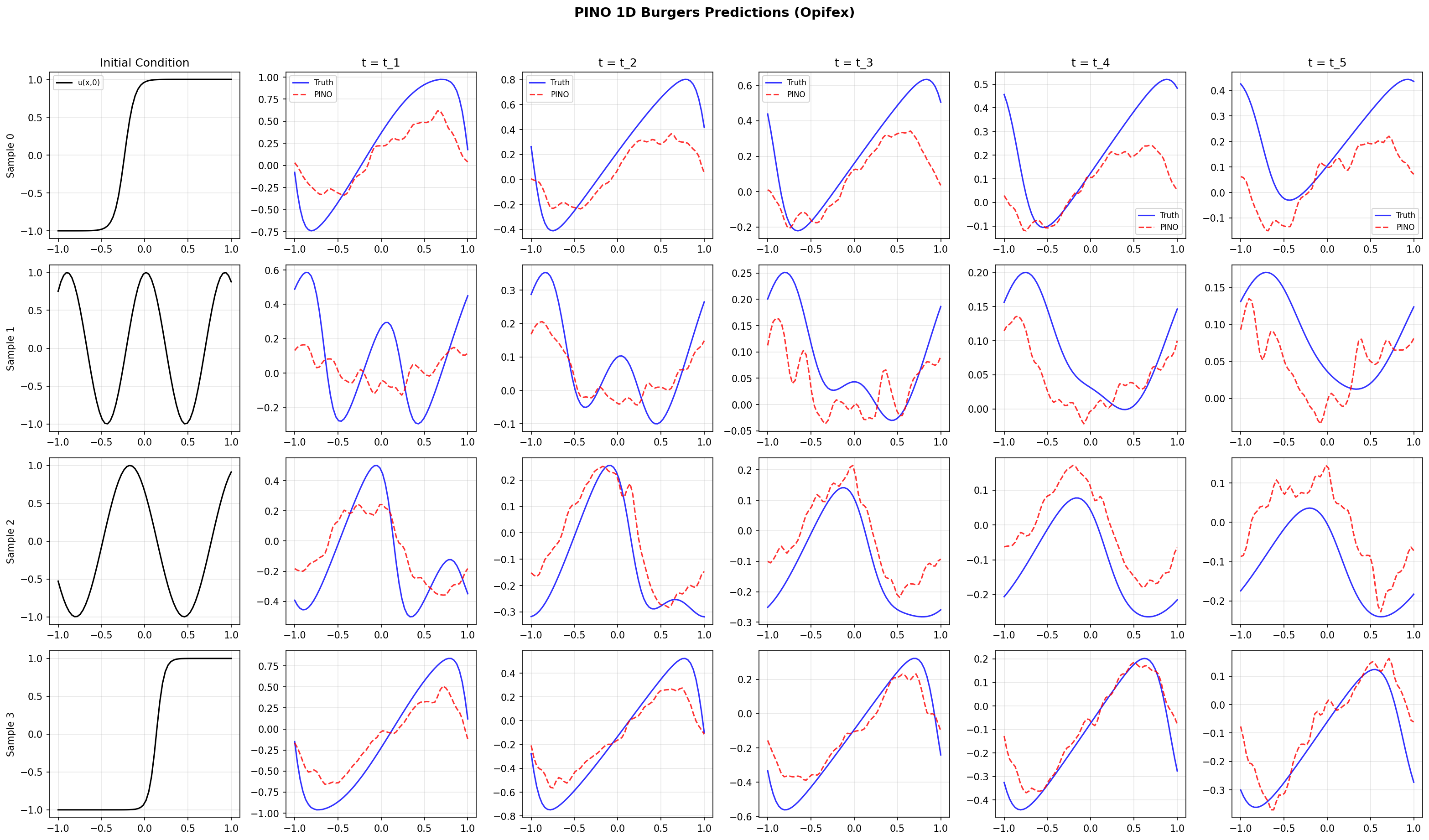
Sample Space-Time Solutions¶

Ground truth, prediction, and absolute error for three test trajectories. The error concentrates near \(t = 0\) — where the initial condition has the sharpest features — and along the convective shock fronts, exactly where Burgers dynamics are hardest.

PINO Predictions

Training Analysis¶

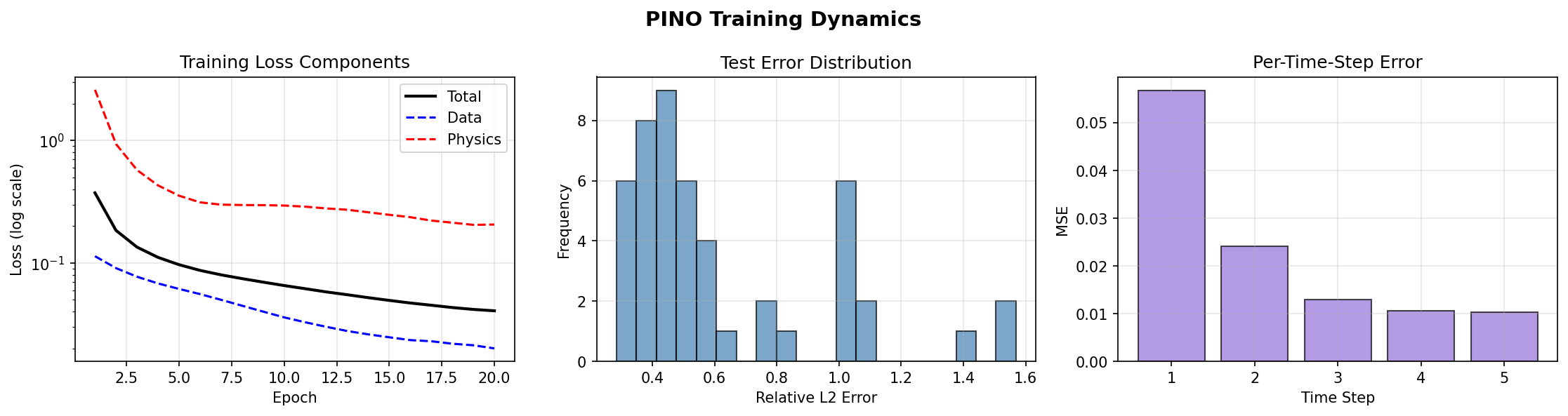
Training Analysis

Results Summary¶

Metric	Value
Test relative L2 (full traj.)	0.0336
Test IC RMS error (t=0 slice)	0.052
Test mean PDE residual (MSE)	0.218
Final total training loss	0.084
Training Time	61s (GPU)
Parameters	4,203,009

The PINO recovers the full space-time Burgers solution operator to about 3.4% relative L2 on held-out trajectories, with the predicted \(t = 0\) slice closely matching the true initial condition.

Next Steps¶

Experiments to Try¶

Vary the loss weights (data / IC / equation) and study the trade-off
Adaptive weighting: swap fixed weights for SoftAdapt or ReLoBRaLo
Denser time grid: increase NUM_TIME for finer temporal resolution
Spectral derivatives: replace finite differences with FFT-based residuals
Varying viscosity: add \(\nu\) as an extra input channel to the operator

Example	Level	What You'll Learn
FNO on Burgers Equation	Intermediate	Data-only FNO baseline
FNO on Darcy Flow	Intermediate	2D elliptic PDE
Burgers PINN	Beginner	Physics-only neural network
TFNO on Darcy Flow	Intermediate	Tensorized FNO with compress.

API Reference¶

FourierNeuralOperator — FNO model class
solve_burgers_spectral — pseudo-spectral Burgers solver

Troubleshooting¶

Training loss freezes early¶

Symptom: the loss stops changing after a few dozen epochs.

Cause: the cosine learning-rate schedule decays over too few steps. It is stepped once per mini-batch update, not per epoch.

Solution: set the decay length to NUM_EPOCHS * n_batches:

schedule = optax.cosine_decay_schedule(LEARNING_RATE, NUM_EPOCHS * n_batches)

High PDE residual relative to the data error¶

Symptom: the test PDE residual is larger than the data relative L2.

Cause: the finite-difference residual amplifies errors near the steep IC and the convective shocks, where the field has large spatial gradients.

Solution: raise EQUATION_WEIGHT, refine the grid (NUM_SPACE, NUM_TIME), or use spectral derivatives for a more accurate residual.

PINO on Burgers Equation¶

Overview¶

The genuine PINO setup¶

What You'll Learn¶

Coming from NeuralOperator (PyTorch)?¶

Files¶

Quick Start¶

Run the Python Script¶

Run the Jupyter Notebook¶

Core Concepts¶

Physics-Informed Loss¶

PINO Architecture¶

Implementation¶

Step 1: Imports and Setup¶

Step 2: Data Generation¶

Step 3: PDE Residual¶

Step 4: Model Creation¶

Step 5: Training¶

Step 6: Evaluation¶

Visualization¶

Sample Space-Time Solutions¶

Training Analysis¶

Results Summary¶

Next Steps¶

Experiments to Try¶

Related Examples¶

API Reference¶

Troubleshooting¶

Training loss freezes early¶

High PDE residual relative to the data error¶