GNO on Darcy Flow

Metadata	Value
Level	Intermediate
Runtime	~2 min (CPU) / ~15s (GPU)
Prerequisites	JAX, Flax NNX, GNN basics
Format	Python + Jupyter
Memory	~500 MB RAM

Overview

This tutorial demonstrates training a Graph Neural Operator (GNO) on the Darcy flow problem. GNO uses message passing neural networks to learn operators on graph-structured data, making it naturally suited for problems with irregular geometries or unstructured meshes.

Unlike Fourier-based operators (FNO, TFNO) that require uniform grids, GNO operates on arbitrary node connectivity patterns. This flexibility comes at the cost of computational efficiency on regular grids, where spectral methods excel. This example shows how to convert regular grid data to graph format and train a GNO.

What You'll Learn

1. Convert 2D grid data to graph representation using grid_to_graph_data()
2. Understand GNO's message passing architecture for operator learning
3. Configure graph connectivity (4-neighbor, 8-neighbor, radius-based)
4. Train a GraphNeuralOperator with custom loss on node features
5. Visualize predictions by converting graph output back to grid format

Coming from NeuralOperator (PyTorch)?

If you are familiar with the neuraloperator library:

NeuralOperator (PyTorch)	Opifex (JAX)
GNOBlock(radius=0.035)	GraphNeuralOperator(node_dim, hidden_dim, ...)
Runtime neighbor search (Open3D)	Pre-computed edge indices
NeighborSearch module	grid_to_graph_data(connectivity=8)
IntegralTransform with MLP kernel	MessagePassingLayer with explicit edge features
Handles variable node counts	Fixed graph structure (batch-friendly)

Key differences:

1. Pre-computed edges: Opifex expects edge indices upfront, enabling JAX's static shapes
2. Explicit edge features: Edge features are computed externally and passed to the model
3. Fixed batch structure: All graphs in a batch must have the same node/edge counts
4. Grid-to-graph utilities: Built-in grid_to_graph_data() for regular grid conversion

Files

• Python Script: examples/neural-operators/gno_darcy.py
• Jupyter Notebook: examples/neural-operators/gno_darcy.ipynb

Quick Start

Run the Python Script

source activate.sh && python examples/neural-operators/gno_darcy.py

Run the Jupyter Notebook

jupyter lab examples/neural-operators/gno_darcy.ipynb

Core Concepts

GNO Architecture

GNO applies message passing neural networks to learn operators on graphs:

graph LR
    subgraph Input
        A["Grid Data<br/>(1, 16, 16)"]
    end

    subgraph Preprocessing["Grid-to-Graph Conversion"]
        B["Flatten to Nodes<br/>(256 nodes)"]
        C["Create Edges<br/>(1860 edges)"]
        D["Compute Edge Features<br/>(relative positions)"]
    end

    subgraph GNO["Graph Neural Operator"]
        E["Input Projection<br/>node_dim → hidden_dim"]
        F["MessagePassingLayer 1"]
        G["MessagePassingLayer 2"]
        H["MessagePassingLayer 3"]
        I["MessagePassingLayer 4"]
        J["Output Projection<br/>hidden_dim → node_dim"]
    end

    subgraph Output
        K["Predicted Nodes<br/>(256 nodes)"]
        L["Reshape to Grid<br/>(1, 16, 16)"]
    end

    A --> B --> C --> D --> E --> F --> G --> H --> I --> J --> K --> L

Message Passing Layer

Each layer computes node updates through three steps:

graph TB
    A["Node Features<br/>(num_nodes, hidden_dim)"] --> B["Get Source Nodes<br/>src_nodes = nodes[edges[:, 0]]"]
    A --> C["Get Target Nodes<br/>dst_nodes = nodes[edges[:, 1]]"]
    D["Edge Features<br/>(num_edges, 2)"] --> E["Concatenate<br/>[src, dst, edge_feat]"]
    B --> E
    C --> E
    E --> F["Message MLP<br/>→ messages"]
    F --> G["Aggregate at Targets<br/>aggregated[dst] += messages"]
    G --> H["Update MLP<br/>[node, aggregated] → updated"]
    A --> H
    H --> I["Residual Connection<br/>+ original"]
    I --> J["Output<br/>(num_nodes, hidden_dim)"]

    style F fill:#e3f2fd,stroke:#1976d2
    style H fill:#fff3e0,stroke:#f57c00

When to Use GNO

Problem Type	GNO	FNO	Recommendation
Regular 2D/3D grids	OK	Best	Use FNO for efficiency
Irregular meshes	Best	N/A	GNO handles any connectivity
Point clouds	Best	N/A	GNO works on unstructured data
Variable geometry	Best	Limited	GNO adapts to node layout
Large regular grids	Slow	Fast	FNO scales better (O(N log N))

Implementation

Step 1: Imports and Setup

import jax
from flax import nnx

from opifex.data.loaders import create_darcy_loader
from opifex.neural.operators.graph import (
    GraphNeuralOperator,
    graph_to_grid,
    grid_to_graph_data,
)

Terminal Output:

======================================================================
Opifex Example: GNO on Darcy Flow
======================================================================
JAX backend: gpu
JAX devices: [CudaDevice(id=0)]
Resolution: 16x16
Training samples: 200, Test samples: 50
Batch size: 16, Epochs: 30
GNO config: hidden_dim=32, layers=4
Graph connectivity: 8-neighbor

Step 2: Data Loading and Graph Conversion

train_loader = create_darcy_loader(
    n_samples=200,
    batch_size=16,
    resolution=16,
    shuffle=True,
    seed=42,
)

# Convert grid data to graph format
train_nodes, train_edges, train_edge_feats = grid_to_graph_data(
    X_train, connectivity=8
)

Terminal Output:

Generating Darcy flow data...
Grid data: X=(16, 1, 16, 16), Y=(16, 1, 16, 16)

Converting grids to graphs...
Node features shape: (16, 256, 3)
Edge indices shape:  (16, 1860, 2)
Edge features shape: (16, 1860, 2)
Num nodes per graph: 256 (16x16)
Num edges per graph: 1860

Step 3: Model Creation

gno = GraphNeuralOperator(
    node_dim=train_nodes.shape[-1],  # 3: value + x + y
    hidden_dim=32,
    num_layers=4,
    edge_dim=train_edge_feats.shape[-1],  # 2: dx, dy
    rngs=nnx.Rngs(42),
)

Terminal Output:

Creating GNO model...
GNO parameters: 25,571

Step 4: Training

opt = nnx.Optimizer(gno, optax.adam(1e-3), wrt=nnx.Param)

@nnx.jit
def train_step(model, opt, nodes, edges, edge_feats, targets):
    def loss_fn(model):
        pred = model(nodes, edges, edge_feats)
        # Compare value channel only (not position encoding)
        return jnp.mean((pred[:, :, 0] - targets[:, :, 0]) ** 2)

    loss, grads = nnx.value_and_grad(loss_fn)(model)
    opt.update(model, grads)
    return loss

Terminal Output:

Training GNO...
  Epoch   1/30: loss=16.764143
  Epoch   5/30: loss=2.551377
  Epoch  10/30: loss=1.369779
  Epoch  15/30: loss=0.550659
  Epoch  20/30: loss=0.372531
  Epoch  25/30: loss=0.302217
  Epoch  30/30: loss=0.195386
Final GNO loss: 1.953856e-01

Step 5: Evaluation

Terminal Output:

Running evaluation...
GNO Results:
  Test MSE:         0.198459
  Relative L2:      17.064571 (min=13.048689, max=23.490587)

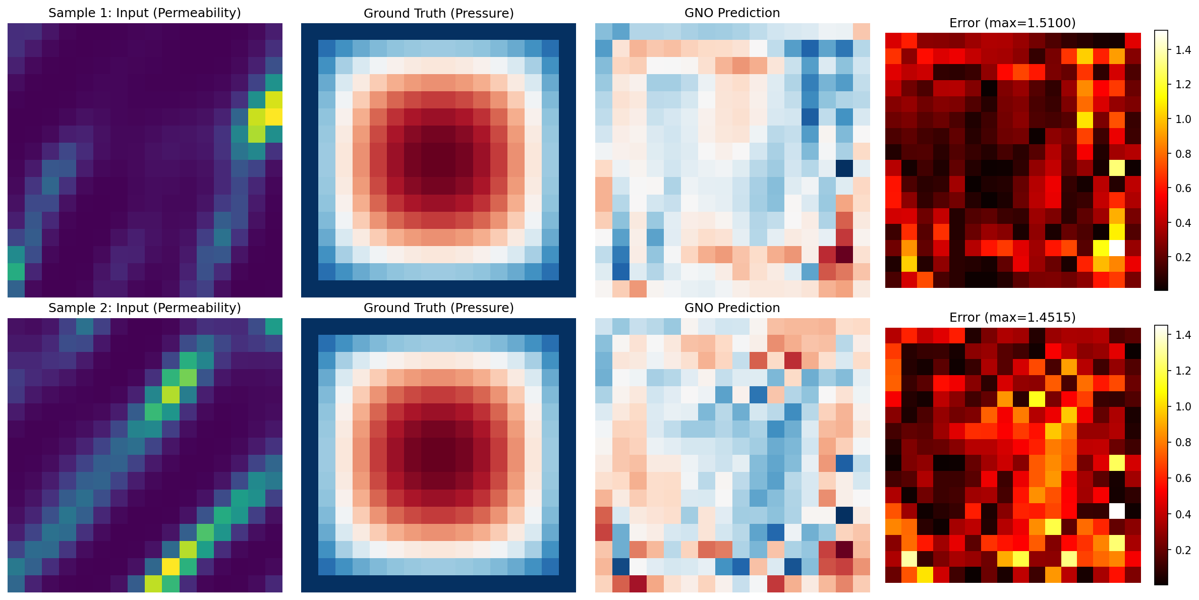
Visualization

Predictions Comparison

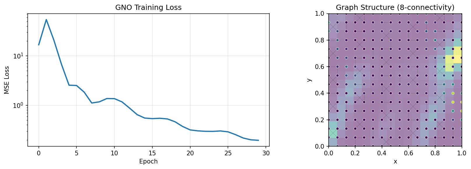
Training and Graph Structure

Results Summary

Metric	GNO
Test MSE	0.198459
Relative L2 Error	17.06
Parameters	25,571
Resolution	16x16

Note: GNO achieves higher MSE than FNO on this regular grid problem because: 1. FNO's spectral convolutions are optimal for uniform grids 2. GNO's message passing is designed for irregular geometries 3. The 16x16 resolution was chosen to keep graph size manageable

GNO excels on problems with non-uniform meshes, complex boundaries, or varying node densities where FNO cannot be applied.

Next Steps

Experiments to Try

1. Increase resolution: Try 32x32 (requires more memory due to O(n^2) edges)
2. Try radius-based connectivity: Use connectivity="radius", radius=1.5
3. Apply to irregular mesh: Load mesh data instead of regular grid
4. Combine with FNO: Use GNO for boundary regions, FNO for interior (GINO approach)

Related Examples

Example	Level	What You'll Learn
FNO on Darcy Flow	Intermediate	Spectral methods (compare MSE)
Local FNO on Darcy	Intermediate	Local + global features
DeepONet on Darcy	Intermediate	Branch-trunk architecture

API Reference

• GraphNeuralOperator - Graph neural operator model
• MeshGraphNet - Encoder-processor-decoder architecture for mesh-based simulation (Pfaff et al., 2021). Reuses MessagePassingLayer internally
• MessagePassingLayer - Individual message passing layer
• grid_to_graph_data - Grid to graph conversion utility
• graph_to_grid - Graph to grid conversion utility
• create_darcy_loader - Darcy flow data loader

Troubleshooting

Memory error with large grids

Symptom: RESOURCE_EXHAUSTED error when increasing resolution.

Cause: 8-connectivity creates O(8n) edges where n = H*W nodes. At 32x32 = 1024 nodes with ~7000 edges, memory usage grows significantly.

Solution: Reduce connectivity or batch size:

# Use 4-connectivity (fewer edges)
node_features, edge_indices, edge_features = grid_to_graph_data(
    grid, connectivity=4
)

# Or reduce batch size
BATCH_SIZE = 8

GNO performs worse than FNO on regular grids

Symptom: Higher MSE/Relative L2 compared to FNO.

Cause: This is expected behavior. GNO is designed for irregular geometries; FNO's spectral convolutions are optimal for regular grids.

Solution: Use FNO for regular grids. Reserve GNO for: - Unstructured meshes - Adaptive refinement regions - Complex boundary geometries - Point cloud data

JIT compilation is slow

Symptom: First forward pass takes a long time.

Cause: Message passing over many edges requires tracing.

Solution: The first call triggers XLA compilation. Subsequent calls are fast. For development, use smaller grids:

RESOLUTION = 8  # Faster compilation for debugging