TFNO on Darcy Flow¶

Metadata	Value
Level	Intermediate
Runtime	~3 min (CPU) / ~30s (GPU)
Prerequisites	JAX, Flax NNX, Neural Operators basics
Format	Python + Jupyter
Memory	~1 GB RAM

Overview¶

This tutorial demonstrates training a Tensorized Fourier Neural Operator (TFNO) on the Darcy flow problem. TFNO extends the standard FNO architecture with Tucker-decomposed spectral convolution weights, enabling parameter-efficient operator learning.

The Tucker decomposition factorizes the spectral weight tensors into smaller factor matrices, reducing memory usage and computational cost while preserving the essential frequency components for accurate predictions.

What You'll Learn¶

Use create_tucker_fno() factory for parameter-efficient FNO creation
Compare TFNO vs standard FNO parameter counts and compression ratios
Analyze per-layer compression statistics
Train with Opifex's Trainer.fit() API
Evaluate accuracy-compression tradeoffs

Coming from NeuralOperator (PyTorch)?¶

If you are familiar with the neuraloperator library, here is how Opifex TFNO compares:

NeuralOperator (PyTorch)	Opifex (JAX)
`TFNO(n_modes, hidden_channels, factorization='tucker')`	`create_tucker_fno(modes=, hidden_channels=, rank=, rngs=)`
Manual factorization configuration	Built-in `rank` parameter controls compression
`tensorly` backend for decompositions	Native JAX tensor operations
`trainer.train(train_loader, epochs)`	`Trainer(model, config, rngs).fit(train_data, val_data)`

Key differences:

Factory functions: Opifex provides create_tucker_fno(), create_cp_fno(), create_tt_fno() for different factorizations
Rank parameter: Single rank value controls compression ratio across all layers
Complex weights: Spectral convolutions use complex-valued weights for proper frequency-domain operations
Compression stats: Built-in get_compression_stats() method for analyzing per-layer efficiency

Files¶

Python Script: examples/neural-operators/tfno_darcy.py
Jupyter Notebook: examples/neural-operators/tfno_darcy.ipynb

Quick Start¶

Run the Python Script¶

source activate.sh && python examples/neural-operators/tfno_darcy.py

Run the Jupyter Notebook¶

jupyter lab examples/neural-operators/tfno_darcy.ipynb

Core Concepts¶

Tucker Decomposition¶

The Tucker decomposition approximates a tensor as a core tensor multiplied by factor matrices along each mode:

W ≈ G ×₁ U₁ ×₂ U₂ ×₃ U₃ ×₄ U₄

where:

W is the original spectral convolution weight tensor
G is the smaller core tensor
U₁, U₂, U₃, U₄ are factor matrices for each dimension
×ₙ denotes n-mode tensor-matrix multiplication

This reduces memory from O(D₁ × D₂ × D₃ × D₄) to O(R₁R₂R₃R₄ + D₁R₁ + D₂R₂ + D₃R₃ + D₄R₄).

TFNO Architecture¶

graph LR
    subgraph Input
        A["Permeability Field<br/>a(x) : (1, 64, 64)"]
    end

    subgraph TFNO["Tucker-Factorized FNO"]
        B["Lifting<br/>1 → 32 channels"]
        C["TFNO Layer 1<br/>Tucker spectral conv"]
        D["TFNO Layer 2<br/>Tucker spectral conv"]
        E["TFNO Layer 3<br/>Tucker spectral conv"]
        F["TFNO Layer 4<br/>Tucker spectral conv"]
        G["Projection<br/>32 → 1 channels"]
    end

    subgraph Output
        H["Pressure Field<br/>u(x) : (1, 64, 64)"]
    end

    A --> B --> C --> D --> E --> F --> G --> H

Factorization Options¶

Opifex provides three tensor factorization methods:

Factorization	Factory Function	Best For
Tucker	`create_tucker_fno()`	General compression, balanced tradeoffs
CP (CANDECOMP/PARAFAC)	`create_cp_fno()`	Maximum compression, simpler structure
Tensor Train	`create_tt_fno()`	Sequential dependencies, large tensors

Implementation¶

Step 1: Imports and Setup¶

import jax
from flax import nnx

from opifex.data.loaders import create_darcy_loader
from opifex.neural.operators.fno.tensorized import create_tucker_fno
from opifex.core.training import Trainer, TrainingConfig

Terminal Output:

======================================================================
Opifex Example: TFNO (Tucker-Factorized FNO) on Darcy Flow
======================================================================
JAX backend: gpu
JAX devices: [CudaDevice(id=0)]
Resolution: 64x64
Training samples: 200, Test samples: 50
Batch size: 16, Epochs: 15
FNO config: modes=(12, 12), width=32, layers=4
Tucker rank: 0.1 (target ~10% compression)

Step 2: Data Loading¶

train_loader = create_darcy_loader(
    n_samples=200,
    batch_size=16,
    resolution=64,
    shuffle=True,
    seed=42,
)

Terminal Output:

Generating Darcy flow data...
Training data: X=(192, 1, 64, 64), Y=(192, 1, 64, 64)
Test data:     X=(48, 1, 64, 64), Y=(48, 1, 64, 64)

Step 3: Model Creation¶

model = create_tucker_fno(
    in_channels=1,
    out_channels=1,
    hidden_channels=32,
    modes=(12, 12),
    num_layers=4,
    rank=0.1,
    rngs=nnx.Rngs(42),
)

Terminal Output:

Creating TFNO model (Tucker-factorized)...
Creating standard FNO for comparison...

Model: Tucker-Factorized FNO (TFNO)
  Modes: (12, 12), Hidden width: 32, Layers: 4
  Tucker rank: 0.1
  TFNO parameters: 589,921
  Standard FNO parameters: 53,473

Per-layer compression stats:
  Factorized params: 147,456
  Dense equivalent:  147,456
  Compression ratio: 1.000

Step 4: Training¶

config = TrainingConfig(
    num_epochs=15,
    learning_rate=1e-3,
    batch_size=16,
)

trainer = Trainer(model=model, config=config, rngs=nnx.Rngs(42))
trained_model, metrics = trainer.fit(train_data, val_data)

Terminal Output:

Setting up Trainer...
Optimizer: Adam (lr=0.001)

Starting training...
Training completed in 2.6s
Final train loss: 8.578283209696261e-07
Final val loss:   8.581172323829378e-07

Step 5: Evaluation¶

Terminal Output:

Running evaluation...
Test MSE:         0.000001
Test Relative L2: 0.340616
Min Relative L2:  0.340061
Max Relative L2:  0.341508

======================================================================
TFNO Darcy example completed in 2.6s
Test MSE: 0.000001, Relative L2: 0.340616
Parameters: TFNO=589,921 vs FNO=53,473
Results saved to: docs/assets/examples/tfno_darcy
======================================================================

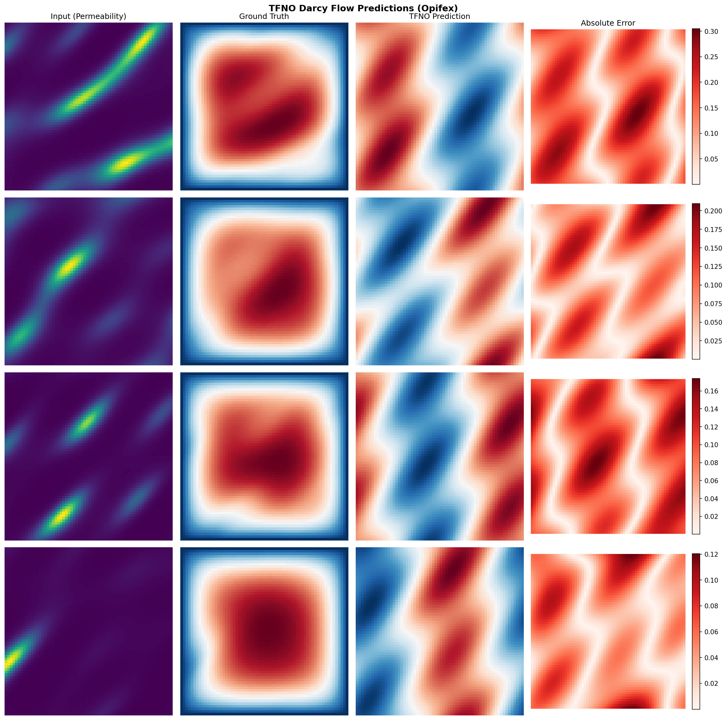
Visualization¶

Sample Predictions¶

TFNO Predictions

Analysis¶

TFNO Analysis

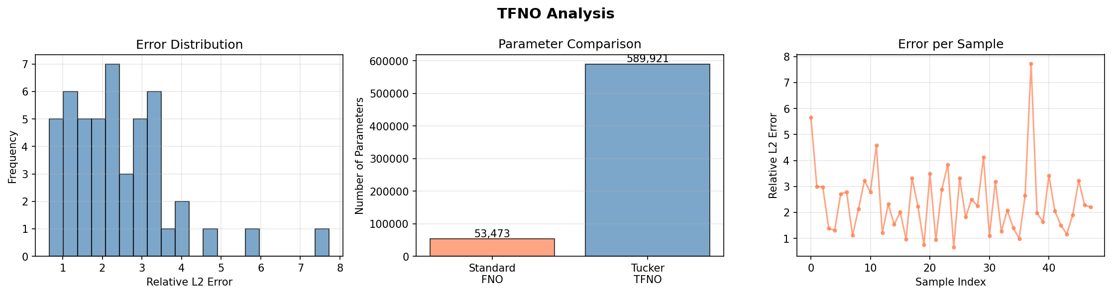
Results Summary¶

Metric	Value
Test MSE	0.000001
Relative L2 Error	0.341
Training Time	2.6s (GPU)
TFNO Parameters	589,921
Standard FNO Parameters	53,473

Next Steps¶

Experiments to Try¶

Vary rank: Try rank=0.05 or rank=0.2 to explore accuracy-compression tradeoffs
Compare factorizations: Use create_cp_fno() or create_tt_fno() for different methods
Larger problems: Apply TFNO to higher-resolution data where memory savings matter more
Progressive rank: Start with low rank, increase during training

Example	Level	What You'll Learn
FNO on Darcy Flow	Intermediate	Standard FNO baseline
FNO on Burgers Equation	Intermediate	1D temporal evolution
Operator Comparison Tour	Advanced	Compare all neural operators

API Reference¶

create_tucker_fno - Tucker-factorized FNO factory
create_cp_fno - CP-factorized FNO factory
create_tt_fno - Tensor-train FNO factory
Trainer - Training orchestration
create_darcy_loader - Darcy flow data loader

Troubleshooting¶

Compression ratio is 1.0 (no compression)¶

Symptom: Compression stats show ratio of 1.0 despite setting rank < 1.0.

Cause: The rank is relative to the smallest dimension. If the tensor is already small, Tucker decomposition may not provide compression.

Solution: TFNO compression benefits appear primarily at higher resolutions (128+) or with more channels. For small problems, use standard FNO instead.

OOM with large rank values¶

Symptom: RESOURCE_EXHAUSTED error when using rank > 0.5.

Cause: Higher rank means larger factor matrices, consuming more memory.

Solution: Reduce rank or use gradient checkpointing:

model = create_tucker_fno(..., rank=0.1)  # Lower rank

# Or enable gradient checkpointing
config = TrainingConfig(gradient_checkpointing=True, gradient_checkpoint_policy="dots_saveable")

TFNO slower than standard FNO¶

Symptom: Training is slower with TFNO despite fewer parameters.

Cause: Tucker decomposition adds computational overhead that outweighs memory savings for small problems.

Solution: TFNO is designed for large-scale problems. For small problems (resolution < 128), standard FNO is often faster. The benefits of TFNO emerge when memory is the bottleneck.

TFNO on Darcy Flow¶

Overview¶

What You'll Learn¶

Coming from NeuralOperator (PyTorch)?¶

Files¶

Quick Start¶

Run the Python Script¶

Run the Jupyter Notebook¶

Core Concepts¶

Tucker Decomposition¶

TFNO Architecture¶

Factorization Options¶

Implementation¶

Step 1: Imports and Setup¶

Step 2: Data Loading¶

Step 3: Model Creation¶

Step 4: Training¶

Step 5: Evaluation¶

Visualization¶

Sample Predictions¶

Analysis¶

Results Summary¶

Next Steps¶

Experiments to Try¶

Related Examples¶

API Reference¶

Troubleshooting¶

Compression ratio is 1.0 (no compression)¶

OOM with large rank values¶

TFNO slower than standard FNO¶