Helmholtz Equation PINN¶

Metadata	Value
Level	Intermediate
Runtime	~2 min (GPU) / ~8 min (CPU)
Prerequisites	JAX, Flax NNX, wave physics
Format	Python + Jupyter
Memory	~800 MB RAM

Overview¶

This tutorial demonstrates solving the 2D Helmholtz equation using a Physics-Informed Neural Network (PINN). The Helmholtz equation arises in acoustics, electromagnetics, seismology, and quantum mechanics as the time-independent form of the wave equation.

This example showcases a hard boundary constraint technique where the network output is multiplied by a function that vanishes on boundaries, automatically satisfying Dirichlet conditions without explicit boundary loss.

What You'll Learn¶

Implement a PINN for the Helmholtz equation with oscillatory solutions
Apply hard boundary constraints using output transforms
Use sinusoidal activation functions for wave-like solutions
Handle high-frequency solutions that challenge spectral bias
Compare hard vs soft boundary enforcement strategies

Coming from DeepXDE?¶

If you are familiar with the DeepXDE library:

DeepXDE	Opifex (JAX)
`dde.geometry.Rectangle([0,0], [1,1])`	`jax.random.uniform(key, (N, 2))` for (x, y)
`dde.grad.hessian(y, x, i=0, j=0)`	`jax.hessian(u_fn)(xy)[0, 0]` for u_xx
`net.apply_output_transform(transform)`	Hard constraint in `__call__` method
`dde.nn.FNN([2]+[150]*3+[1], "sin")`	Custom `HelmholtzPINN` with `jnp.sin` activation
`model.compile("adam", lr=1e-3)`	`nnx.Optimizer(pinn, optax.adam(lr), wrt=nnx.Param)`

Key differences:

Hard constraint in model: BC enforcement built into network forward pass
Sin activation: jnp.sin(layer(h)) instead of tanh for oscillatory solutions
No BC loss: With hard constraints, only PDE residual is needed
Zero boundary error: Hard constraint achieves machine precision on boundaries

Files¶

Python Script: examples/pinns/helmholtz.py
Jupyter Notebook: examples/pinns/helmholtz.ipynb

Quick Start¶

Run the Python Script¶

source activate.sh && python examples/pinns/helmholtz.py

Run the Jupyter Notebook¶

jupyter lab examples/pinns/helmholtz.ipynb

Core Concepts¶

Helmholtz Equation¶

The Helmholtz equation is an elliptic PDE:

\[-\nabla^2 u - k_0^2 u = f(x, y)\]

Component	This Example
Domain	\([0, 1] \times [0, 1]\)
Wave number	\(k_0 = 4\pi\) (2 wavelengths per unit)
Source term	\(f = k_0^2 \sin(k_0 x) \sin(k_0 y)\)
Boundary conditions	\(u = 0\) on \(\partial\Omega\) (Dirichlet)
Analytical solution	\(u = \sin(k_0 x) \sin(k_0 y)\)

Hard Boundary Constraint¶

Instead of adding a boundary loss term, we modify the network output:

\[u_{PINN}(x, y) = x(1-x) \cdot y(1-y) \cdot \hat{u}_{NN}(x, y)\]

This ensures \(u = 0\) on all boundaries exactly because: - At \(x = 0\) or \(x = 1\): \(x(1-x) = 0\) - At \(y = 0\) or \(y = 1\): \(y(1-y) = 0\)

PINN Architecture¶

graph TB
    subgraph Input["Collocation Points"]
        A["Domain Points<br/>(x, y) in [0,1]²"]
    end

    subgraph PINN["Neural Network with Hard Constraint"]
        B["Linear + sin<br/>150 units"]
        C["Linear + sin<br/>150 units"]
        D["Linear + sin<br/>150 units"]
        E["Linear<br/>1 unit"]
        F["Hard BC Mask<br/>x(1-x)·y(1-y)"]
        G["u = mask × u_hat"]
    end

    subgraph Loss["Physics-Informed Loss"]
        H["PDE Residual Only<br/>|-∇²u - k₀²u - f|²"]
    end

    A --> B --> C --> D --> E --> F --> G --> H

    style F fill:#e8f5e9,stroke:#388e3c
    style H fill:#e3f2fd,stroke:#1976d2

Implementation¶

Step 1: Imports and Configuration¶

import jax
import jax.numpy as jnp
import optax
from flax import nnx

Terminal Output:

======================================================================
Opifex Example: Helmholtz Equation PINN
======================================================================
JAX backend: gpu
JAX devices: [CudaDevice(id=0)]
Wave number: k0 = 12.5664 (n=2 modes)
Wavelength: 0.5000
Domain: [0, 1] x [0, 1]
Collocation: 2500 domain, 400 boundary
Network: [2] + [150, 150, 150] + [1]
Hard BC constraint: True
Training: 5000 epochs @ lr=0.001

Step 2: Define the Problem¶

N_MODES = 2  # Number of wavelengths in each direction
K0 = 2.0 * jnp.pi * N_MODES  # Wave number k0 = 4*pi

def exact_solution(xy):
    x, y = xy[:, 0], xy[:, 1]
    return jnp.sin(K0 * x) * jnp.sin(K0 * y)

def source_term(xy):
    x, y = xy[:, 0], xy[:, 1]
    return K0**2 * jnp.sin(K0 * x) * jnp.sin(K0 * y)

Terminal Output:

Helmholtz equation: -nabla^2(u) - k0^2 * u = f(x,y)
  Wave number: k0 = 2*pi*2 = 12.5664
  Source term: f = k0^2 * sin(k0*x) * sin(k0*y)
  Boundary: u = 0 (Dirichlet)
  Analytical solution: u = sin(k0*x) * sin(k0*y)

Step 3: Create PINN with Hard Constraint¶

class HelmholtzPINN(nnx.Module):
    def __init__(self, hidden_dims: list[int], *, rngs: nnx.Rngs):
        layers = []
        in_features = 2
        for hidden_dim in hidden_dims:
            layers.append(nnx.Linear(in_features, hidden_dim, rngs=rngs))
            in_features = hidden_dim
        layers.append(nnx.Linear(in_features, 1, rngs=rngs))
        self.layers = nnx.List(layers)

    def __call__(self, xy):
        h = xy
        for layer in self.layers[:-1]:
            h = jnp.sin(layer(h))  # sin activation
        u_hat = self.layers[-1](h)

        # Hard constraint: u = x*(1-x) * y*(1-y) * u_hat
        x, y = xy[:, 0:1], xy[:, 1:2]
        bc_mask = x * (1 - x) * y * (1 - y)
        return bc_mask * u_hat

Terminal Output:

Creating PINN model...
PINN parameters: 45,901

Step 4: Training (PDE Loss Only)¶

def total_loss(pinn, xy_dom, xy_bc, lambda_bc=100.0):
    loss_pde = pde_loss(pinn, xy_dom)
    # No boundary loss needed with hard constraint!
    return loss_pde

Terminal Output:

Training PINN...
  Epoch     1/5000: loss=6.029034e+03
  Epoch  1000/5000: loss=9.683103e+01
  Epoch  2000/5000: loss=3.790305e+01
  Epoch  3000/5000: loss=1.175391e+01
  Epoch  4000/5000: loss=8.398210e+00
  Epoch  5000/5000: loss=3.463675e+00
Final loss: 3.463675e+00

Step 5: Evaluation¶

Terminal Output:

Evaluating PINN...
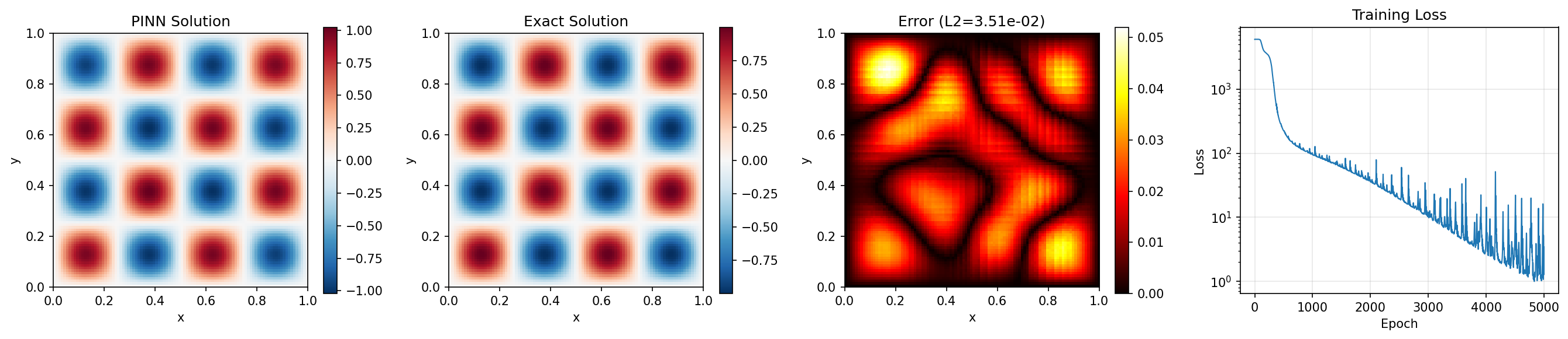
Relative L2 error:   3.506146e-02
Maximum point error: 5.202329e-02
Mean point error:    1.372658e-02
Mean PDE residual:   1.556803e+00
Boundary error:      0.000000e+00

Note the boundary error is exactly zero thanks to the hard constraint!

Visualization¶

Solution Comparison¶

Helmholtz Solution

Cross-Sections¶

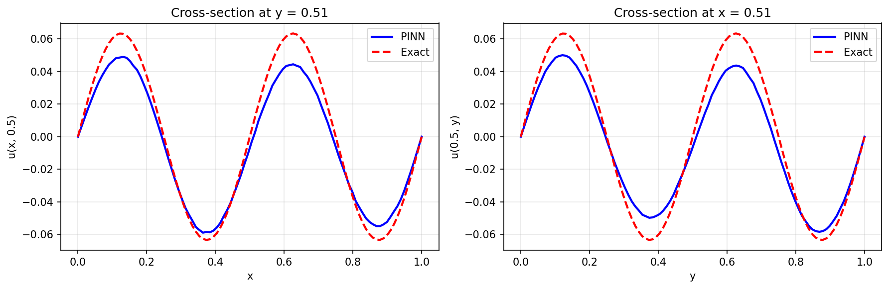
Cross-sections

Results Summary¶

Metric	Value
Final Loss	3.46
Relative L2 Error	3.51%
Maximum Point Error	5.20e-02
Mean Point Error	1.37e-02
Mean PDE Residual	1.56
Boundary Error	0.0
Parameters	45,901
Training Epochs	5,000

Next Steps¶

Experiments to Try¶

More modes: Try \(n = 4\) or \(n = 8\) for higher frequency solutions
Soft constraint: Compare accuracy with USE_HARD_CONSTRAINT = False
Different activations: Try tanh (will struggle with oscillations)
More epochs: Train for 20,000+ epochs for lower L2 error
Fourier features: Add input encoding for high-frequency modes

Example	Level	What You'll Learn
Poisson Equation	Intermediate	Elliptic without wave behavior
Wave Equation	Intermediate	Time-dependent wave physics
Navier-Stokes	Advanced	Multi-output coupled PDEs

API Reference¶

nnx.Linear - Linear layer
nnx.Optimizer - Optimizer wrapper
jax.hessian - Hessian computation

Troubleshooting¶

Loss very high with oscillatory solution¶

Symptom: Loss stays at \(10^3\) or higher even after training.

Cause: tanh activation can't represent high-frequency oscillations (spectral bias).

Solution: Use sin activation as shown, or add Fourier feature encoding:

# Sin activation (recommended for oscillatory solutions)
h = jnp.sin(layer(h))

# Or Fourier features
def fourier_features(xy, k=4):
    x, y = xy[:, 0:1], xy[:, 1:2]
    features = [x, y]
    for i in range(1, k+1):
        features.extend([
            jnp.sin(2*jnp.pi*i*x), jnp.cos(2*jnp.pi*i*x),
            jnp.sin(2*jnp.pi*i*y), jnp.cos(2*jnp.pi*i*y)
        ])
    return jnp.concatenate(features, axis=-1)

Hard constraint causes training instability¶

Symptom: Loss fluctuates wildly or NaN values appear.

Cause: The boundary mask squashes gradients near boundaries.

Solution: Use slightly offset boundaries in mask, or use soft constraint:

# Soft boundary mask (avoids exactly zero gradients)
eps = 0.01
bc_mask = (x + eps) * (1 - x + eps) * (y + eps) * (1 - y + eps)

Solution has wrong number of oscillations¶

Symptom: PINN shows fewer peaks than expected.

Cause: Network capacity insufficient for given \(k_0\).

Solution: Increase network width or add more layers:

# Wider network for high k0
HIDDEN_DIMS = [256, 256, 256, 256]

Helmholtz Equation PINN¶

Overview¶

What You'll Learn¶

Coming from DeepXDE?¶

Files¶

Quick Start¶

Run the Python Script¶

Run the Jupyter Notebook¶

Core Concepts¶

Helmholtz Equation¶

Hard Boundary Constraint¶

PINN Architecture¶

Implementation¶

Step 1: Imports and Configuration¶

Step 2: Define the Problem¶

Step 3: Create PINN with Hard Constraint¶

Step 4: Training (PDE Loss Only)¶

Step 5: Evaluation¶

Visualization¶

Solution Comparison¶

Cross-Sections¶

Results Summary¶

Next Steps¶

Experiments to Try¶

Related Examples¶

API Reference¶

Troubleshooting¶

Loss very high with oscillatory solution¶

Hard constraint causes training instability¶

Solution has wrong number of oscillations¶