Advection Equation PINN

Metadata	Value
Level	Intermediate
Runtime	~2 min (GPU) / ~8 min (CPU)
Prerequisites	JAX, Flax NNX, basic calculus
Format	Python + Jupyter
Memory	~500 MB RAM

Overview

This tutorial demonstrates solving the 1D linear advection equation using a Physics-Informed Neural Network (PINN). The advection equation describes pure transport of a quantity by a flow field without diffusion.

This is a fundamental hyperbolic PDE where information propagates along characteristic lines. PINNs must learn to track the traveling wave solution.

What You'll Learn

1. Implement a PINN for first-order hyperbolic PDEs
2. Handle inflow boundary conditions for transport problems
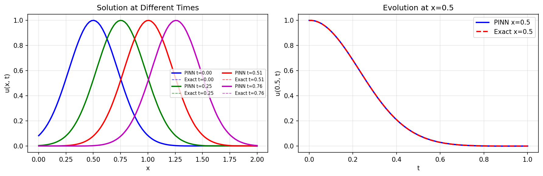
3. Capture traveling wave solutions
4. Understand the characteristic method interpretation

Coming from DeepXDE?

DeepXDE	Opifex (JAX)
dde.geometry.GeometryXTime(geom, time)	jnp.column_stack([x, t]) for (x, t)
dde.icbc.DirichletBC for inflow	Custom inflow_loss() function
dde.icbc.IC for initial condition	Custom initial_loss() function
model.train(iterations=10000)	10000 epochs with Adam optimizer

Key differences:

1. Explicit gradients: Use jax.grad for automatic differentiation
2. Inflow BC: Handled via loss term matching analytical solution
3. No special geometry: Simple uniform sampling in space-time domain

Files

• Python Script: examples/pinns/advection.py
• Jupyter Notebook: examples/pinns/advection.ipynb

Quick Start

Run the Python Script

source activate.sh && python examples/pinns/advection.py

Run the Jupyter Notebook

jupyter lab examples/pinns/advection.ipynb

Core Concepts

Advection Equation

\[\frac{\partial u}{\partial t} + c \frac{\partial u}{\partial x} = 0\]

Component	This Example
Domain	\(x \in [0, 2]\), \(t \in [0, 1]\)
Velocity	\(c = 1\)
IC	Gaussian pulse \(u(x,0) = e^{-(x-0.5)^2/0.1}\)
BC	Inflow condition at \(x = 0\)
Solution	\(u(x,t) = u_0(x - ct)\) (traveling wave)

Physical Interpretation

• Transport: Information propagates along characteristics \(x - ct = \text{const}\)
• No diffusion: The solution maintains its shape as it travels
• Inflow BC: At \(x=0\), we specify incoming values from the left boundary

Implementation

Step 1: Imports and Configuration

import jax
import jax.numpy as jnp
import optax
from flax import nnx

Terminal Output:

======================================================================
Opifex Example: Advection Equation PINN
======================================================================
JAX backend: gpu
JAX devices: [CudaDevice(id=0)]
Advection velocity: c = 1.0
Domain: x in [0.0, 2.0], t in [0.0, 1.0]
Collocation: 5000 domain, 200 inflow, 400 initial
Network: [2] + [40, 40, 40] + [1]
Training: 10000 epochs @ lr=0.001

Step 2: Define the Problem

C = 1.0  # Advection velocity

def exact_solution(x, t):
    """Exact solution: Gaussian pulse traveling with speed c."""
    x0 = 0.5
    sigma2 = 0.1
    return jnp.exp(-((x - C * t - x0) ** 2) / sigma2)

def initial_condition(x):
    """Initial condition: Gaussian pulse centered at x=0.5."""
    return jnp.exp(-((x - 0.5) ** 2) / 0.1)

def inflow_condition(t):
    """Inflow BC at x=0: u(0, t) matches analytical solution."""
    return jnp.exp(-((-C * t - 0.5) ** 2) / 0.1)

Terminal Output:

Advection equation: du/dt + c*du/dx = 0
  Velocity: c = 1.0
  IC: u(x, 0) = exp(-(x-0.5)^2 / 0.1)
  BC: u(0, t) = exact solution at inflow
  Solution: u(x, t) = u0(x - c*t)

Step 3: Create the PINN

class AdvectionPINN(nnx.Module):
    def __init__(self, hidden_dims: list[int], *, rngs: nnx.Rngs):
        super().__init__()
        layers = []
        in_features = 2  # (x, t)

        for hidden_dim in hidden_dims:
            layers.append(nnx.Linear(in_features, hidden_dim, rngs=rngs))
            in_features = hidden_dim

        layers.append(nnx.Linear(in_features, 1, rngs=rngs))
        self.layers = nnx.List(layers)

    def __call__(self, xt: jax.Array) -> jax.Array:
        h = xt
        for layer in self.layers[:-1]:
            h = jnp.tanh(layer(h))
        return self.layers[-1](h)

pinn = AdvectionPINN(hidden_dims=[40, 40, 40], rngs=nnx.Rngs(42))

Terminal Output:

Creating PINN model...
PINN parameters: 3,441

Step 4: Generate Collocation Points

key = jax.random.PRNGKey(42)
keys = jax.random.split(key, 4)

# Domain interior points
x_domain = jax.random.uniform(keys[0], (N_DOMAIN,), minval=X_MIN, maxval=X_MAX)
t_domain = jax.random.uniform(keys[1], (N_DOMAIN,), minval=T_MIN, maxval=T_MAX)
xt_domain = jnp.column_stack([x_domain, t_domain])

# Inflow boundary (x = 0)
t_inflow = jax.random.uniform(keys[2], (N_BOUNDARY,), minval=T_MIN, maxval=T_MAX)
xt_inflow = jnp.column_stack([jnp.zeros(N_BOUNDARY), t_inflow])
u_inflow = inflow_condition(t_inflow)

# Initial condition (t = 0)
x_initial = jax.random.uniform(keys[3], (N_INITIAL,), minval=X_MIN, maxval=X_MAX)
xt_initial = jnp.column_stack([x_initial, jnp.zeros(N_INITIAL)])
u_initial = initial_condition(x_initial)

Terminal Output:

Generating collocation points...
Domain points:   (5000, 2)
Inflow points:   (200, 2)
Initial points:  (400, 2)

Step 5: Define Physics-Informed Loss

def compute_pde_residual(pinn, xt):
    """Compute advection PDE residual: u_t + c*u_x = 0."""

    def u_scalar(xt_single):
        return pinn(xt_single.reshape(1, 2)).squeeze()

    def residual_single(xt_single):
        grad_u = jax.grad(u_scalar)(xt_single)
        u_x = grad_u[0]
        u_t = grad_u[1]
        return u_t + C * u_x

    return jax.vmap(residual_single)(xt)

def total_loss(pinn, xt_dom, xt_ic, u_ic, xt_in, u_in, lambda_bc=10.0):
    loss_pde = pde_loss(pinn, xt_dom)
    loss_ic = initial_loss(pinn, xt_ic, u_ic)
    loss_in = inflow_loss(pinn, xt_in, u_in)
    return loss_pde + lambda_bc * (loss_ic + loss_in)

Step 6: Training

opt = nnx.Optimizer(pinn, optax.adam(LEARNING_RATE), wrt=nnx.Param)

@nnx.jit
def train_step(pinn, opt, xt_dom, xt_ic, u_ic, xt_in, u_in):
    def loss_fn(model):
        return total_loss(model, xt_dom, xt_ic, u_ic, xt_in, u_in)

    loss, grads = nnx.value_and_grad(loss_fn)(pinn)
    opt.update(pinn, grads)
    return loss

for epoch in range(EPOCHS):
    loss = train_step(pinn, opt, xt_domain, xt_initial, u_initial, xt_inflow, u_inflow)

Terminal Output:

Training PINN...
  Epoch     1/10000: loss=3.735486e+00
  Epoch  2000/10000: loss=5.986348e-04
  Epoch  4000/10000: loss=1.633124e-04
  Epoch  6000/10000: loss=1.010060e-04
  Epoch  8000/10000: loss=1.360641e-04
  Epoch 10000/10000: loss=6.163503e-06
Final loss: 6.163503e-06

Step 7: Evaluation

Terminal Output:

Evaluating PINN...
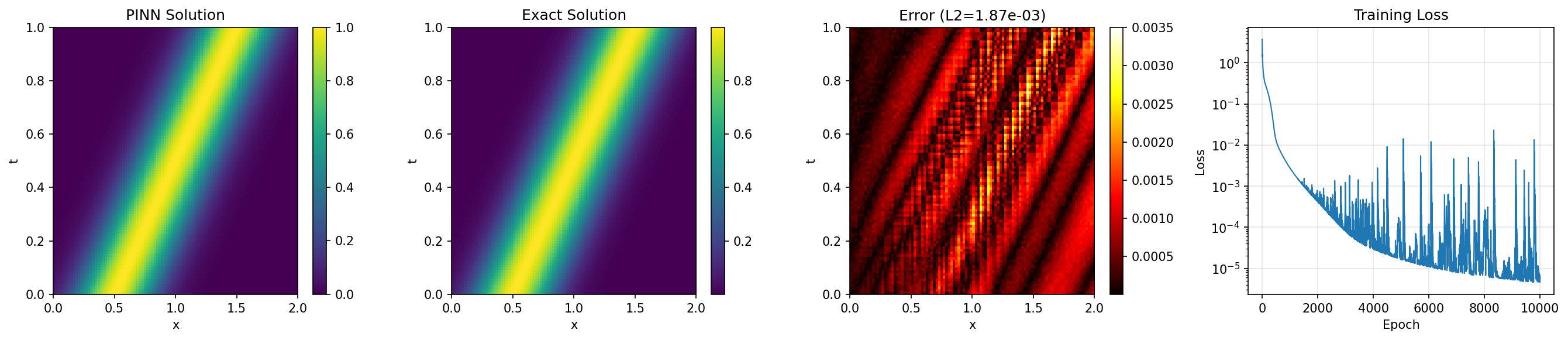
Relative L2 error:   1.866364e-03
Maximum point error: 3.505945e-03
Mean point error:    6.586521e-04
Mean PDE residual:   1.024557e-03

Visualization

Results Summary

Metric	Value
Final Loss	6.16e-06
Relative L2 Error	0.19%
Maximum Point Error	3.51e-03
Mean Point Error	6.59e-04
Mean PDE Residual	1.02e-03
Parameters	3,441
Training Epochs	10,000

Next Steps

Experiments to Try

1. Vary velocity: Try \(c = 2\) or \(c = 0.5\) to see different propagation speeds
2. Different IC: Use a step function or sinusoidal initial condition
3. Longer time: Extend domain to \(t \in [0, 2]\) to track the wave further
4. Higher resolution: Increase collocation points for better accuracy

Related Examples

Example	Level	What You'll Learn
Burgers Equation	Intermediate	Nonlinear advection-diffusion
Wave Equation	Intermediate	Second-order hyperbolic
Heat Equation	Beginner	Pure diffusion (parabolic)

Troubleshooting

Issue	Solution
Poor tracking at late times	Increase training epochs or add more collocation points near later times
Oscillations near boundaries	Check inflow condition matches analytical solution exactly
Slow convergence	Try learning rate scheduling or increase lambda_bc weight