Full U-FNO for Turbulence Modeling
| Metadata | Value |
|---|---|
| Level | Advanced |
| Runtime | ~5 min (CPU) / ~12 sec (GPU) |
| Prerequisites | JAX, Flax NNX, Multi-scale Analysis, Energy Conservation |
| Format | Python + Jupyter |
| Memory | ~2 GB RAM |
Overview
This example demonstrates training a U-Net enhanced Fourier Neural Operator (U-FNO) for
multi-scale 2D Navier-Stokes turbulence modeling using the Opifex framework. The U-FNO
combines the hierarchical encoder-decoder structure of U-Net with Fourier spectral
convolutions, enabling the network to capture turbulent dynamics across multiple spatial
scales simultaneously. The operator maps the initial velocity field (u, v) to the
final-time velocity field of an incompressible Navier-Stokes flow.
The key feature of this example is physics-aware training with custom energy conservation
loss. Rather than relying on generic MSE loss alone, we register a custom loss function
via trainer.custom_losses that penalizes deviations in predicted kinetic energy from the
ground truth -- a physically meaningful constraint for turbulence modeling.
The pipeline covers: loading 2D Navier-Stokes turbulence data via
create_navier_stokes_loader (datarax), augmenting inputs with GridEmbedding2D for
spatial positional encoding, creating the model with create_turbulence_ufno factory,
training with Trainer.fit() plus custom energy loss, and full evaluation with multi-scale
spectral analysis of the velocity-magnitude field.
What You'll Learn
- Build a U-FNO with
create_turbulence_ufnoandGridEmbedding2Dfor positional encoding - Register custom physics-aware loss via
trainer.custom_losses["energy"] - Train with Opifex's
Trainer.fit()API combining MSE and energy conservation - Analyze multi-scale frequency content and energy spectra of predictions
- Evaluate energy conservation, per-sample error distributions, and prediction quality
Coming from NeuralOperator (PyTorch)?
| NeuralOperator (PyTorch) | Opifex (JAX) |
|---|---|
UFNO(n_modes, hidden_channels, uno_n_modes, ...) |
create_turbulence_ufno(in_channels=, out_channels=, rngs=) |
| Manual grid coordinate concatenation | GridEmbedding2D(in_channels=, grid_boundaries=) |
torch.utils.data.DataLoader(dataset) |
create_navier_stokes_loader(...) (datarax PDELoaders) |
Manual energy loss + loss.backward() |
trainer.custom_losses["energy"] = fn + trainer.fit() |
model.to(device) |
Automatic device placement via JAX |
Key differences:
- Factory function:
create_turbulence_ufnopre-configures the U-FNO with multi-scale architecture for turbulence problems - Custom loss API: Register physics losses via
trainer.custom_lossesdict -- no manual gradient computation needed - Explicit PRNG: JAX's
rngs=nnx.Rngs(42)for reproducible model initialization - XLA compilation: Automatic JIT compilation during
Trainer.fit()for GPU/TPU acceleration - Frozen loaders:
create_navier_stokes_loaderreturns aPDELoadersobject exposing pre-split.train/.valdatarax pipelines
Files
- Python Script:
examples/neural-operators/ufno_turbulence.py - Jupyter Notebook:
examples/neural-operators/ufno_turbulence.ipynb
Quick Start
Run the Python Script
Run the Jupyter Notebook
Core Concepts
U-Net Fourier Neural Operator (U-FNO)
The U-FNO enhances the standard FNO with a hierarchical encoder-decoder architecture with skip connections between resolution levels. While a vanilla FNO applies spectral convolutions at a single spatial resolution, the U-FNO processes the field at multiple resolutions through downsampling and upsampling stages with skip connections. This multi-scale design is especially effective for turbulence, where energy cascades across spatial scales.
graph LR
    subgraph Input
        A["Initial Velocity (u, v)<br/>+ Grid Coords<br/>(4 x 64 x 64)"]
    end

    subgraph Encoder["U-FNO Encoder"]
        B["Spectral Layer<br/>@ 64x64"]
        C["Downsample<br/>+ Spectral Layer<br/>@ 32x32"]
    end

    subgraph Decoder["U-FNO Decoder"]
        D["Upsample<br/>+ Spectral Layer<br/>@ 64x64"]
    end

    subgraph Output
        E["Final Velocity (u, v)<br/>(2 x 64 x 64)"]
    end

    A --> B --> C --> D --> E
    B -->|"Skip Connection"| D

    style A fill:#e3f2fd
    style E fill:#c8e6c9
    style C fill:#fff3e0
Each spectral layer at each resolution performs:
- FFT: Transform to Fourier space
- Spectral convolution: Learned weights on truncated Fourier modes
- Inverse FFT: Back to spatial domain
- Skip connection: Add local linear transform
2D Navier-Stokes Turbulence
The incompressible 2D Navier-Stokes equations describe turbulent fluid flow:
| Variable | Meaning | Role |
|---|---|---|
| \(\mathbf{u}(x, t) = (u, v)\) | Velocity field | Prognostic variable (2 channels) |
| \(p\) | Pressure | Enforces incompressibility |
| \(\nu\) | Viscosity | Controls turbulence intensity |
| \(\nabla^2\) | Laplacian | Diffusion operator |
Lower viscosity values produce more turbulent (chaotic) flows. The synthetic data uses viscosity in range [0.001, 0.005] to generate highly turbulent regimes. The model learns to map the initial velocity field \((u, v)\) to the final-time velocity field \((u, v)\).
Grid Embedding for Positional Encoding
GridEmbedding2D appends normalized spatial coordinates (x, y) as additional input
channels. For turbulence modeling, this provides the network with positional context,
helping it learn spatially varying dynamics. A 2-channel velocity field \((u, v)\) becomes a
4-channel tensor (u + v + x-coord + y-coord) after embedding.
Implementation
Step 1: Imports and Setup
import time
import warnings
from pathlib import Path

warnings.filterwarnings("ignore")

import jax
import jax.numpy as jnp
import matplotlib.pyplot as plt
import numpy as np
from flax import nnx

from opifex.core.training import Trainer, TrainingConfig
from opifex.data.loaders.factory import create_navier_stokes_loader
from opifex.neural.operators.common.embeddings import GridEmbedding2D
from opifex.neural.operators.fno.ufno import create_turbulence_ufno
Terminal Output:
======================================================================
Opifex Example: Full U-FNO for 2D Navier-Stokes Turbulence Modeling
======================================================================
JAX backend: gpu
JAX devices: [CudaDevice(id=0)]
Step 2: Configuration
Define experiment parameters as simple variables:
resolution = 64
n_train = 300
n_test = 60
batch_size = 16
num_epochs = 5
learning_rate = 1e-3
in_channels = 2  # (u, v) velocity components
out_channels = 2  # (u, v) velocity components
seed = 42

output_dir = Path("docs/assets/examples/ufno_turbulence")
output_dir.mkdir(parents=True, exist_ok=True)
Terminal Output:
| Hyperparameter | Value | Purpose |
|---|---|---|
resolution |
64 | Spatial grid resolution (64x64) |
n_train / n_test |
300 / 60 | Training and test samples |
batch_size |
16 | Samples per training batch |
num_epochs |
5 | Training epochs |
learning_rate |
1e-3 | Adam optimizer learning rate |
in_channels / out_channels |
2 / 2 | Velocity field \((u, v)\) in/out |
Step 3: Data Loading with datarax
The create_navier_stokes_loader generates synthetic 2D Navier-Stokes turbulence data and
returns a frozen PDELoaders object with pre-split .train / .val datarax pipelines.
Batches are channels-first dicts where input and output are each shaped (batch, 2, H, W)
-- the 2 channels are the (u, v) velocity components (initial velocity in, final velocity out).
n_samples = n_train + n_test
loaders = create_navier_stokes_loader(
    n_samples=n_samples,
    batch_size=batch_size,
    resolution=resolution,
    viscosity_range=(0.001, 0.005),
    time_range=(0.0, 1.0),
    val_fraction=n_test / n_samples,
    seed=seed,
)

def _collect(pipeline: object) -> tuple[np.ndarray, np.ndarray]:
    """Materialize a datarax pipeline into channels-first (N, 2, H, W) arrays."""
    inputs, outputs = [], []
    for batch in pipeline:
        inputs.append(np.asarray(batch["input"]))
        outputs.append(np.asarray(batch["output"]))
    return np.concatenate(inputs, axis=0), np.concatenate(outputs, axis=0)

x_train, y_train = _collect(loaders.train)
x_test, y_test = _collect(loaders.val)
Terminal Output:
Loading 2D Navier-Stokes turbulence data via datarax...
Train: X=(304, 2, 64, 64), Y=(304, 2, 64, 64)
Test:  X=(64, 2, 64, 64), Y=(64, 2, 64, 64)
Frozen PDELoaders
create_navier_stokes_loader returns a PDELoaders object that pre-splits the data
into .train and .val datarax pipelines according to val_fraction. Each batch is a
channels-first dict with input / output shaped (batch, 2, H, W) -- already matching
the model's two-channel (u, v) velocity layout, so no reshaping is required.
Step 4: Model Creation with Grid Embedding
Create a GridEmbedding2D to inject spatial coordinates and the U-FNO model via the
create_turbulence_ufno factory:
grid_embedding = GridEmbedding2D(
    in_channels=in_channels, grid_boundaries=[[0.0, 1.0], [0.0, 1.0]])

model = create_turbulence_ufno(
    in_channels=grid_embedding.out_channels,
    out_channels=out_channels, rngs=nnx.Rngs(seed))
Terminal Output:
Creating U-FNO model with grid embedding...
GridEmbedding2D: 2 -> 4 channels
U-FNO: 4 -> 2 channels
Model parameters: 240,130,562
Step 5: Apply Grid Embedding to Data
We pre-apply the grid embedding to all data before training so Trainer.fit() works
with the embedded inputs directly. This avoids recomputing the embedding every epoch.
def apply_embedding(x_data, embedding):
    """Apply grid embedding: (B, C, H, W) -> embed -> (B, C+2, H, W)."""
    x_grid = jnp.moveaxis(jnp.array(x_data), 1, -1)  # (B, H, W, C)
    x_embedded = embedding(x_grid)                      # (B, H, W, C+2)
    return np.array(jnp.moveaxis(x_embedded, -1, 1))    # (B, C+2, H, W)

x_train_emb = apply_embedding(x_train, grid_embedding)
x_test_emb = apply_embedding(x_test, grid_embedding)
Terminal Output:
Why Pre-Apply Grid Embedding?
GridEmbedding2D expects channels-last format (B, H, W, C) while the U-FNO uses
channels-first (B, C, H, W). By pre-applying the embedding and converting back to
channels-first, we avoid layout conversions inside the training loop. The grid
coordinates are spatial constants that don't change between epochs.
Step 6: Training with Custom Energy Loss
The key physics feature: register an energy conservation loss that penalizes deviations
between predicted and target kinetic energy. The trainer.custom_losses dict allows
adding any number of physics-informed losses that are automatically included in the
training objective.
config = TrainingConfig(
    num_epochs=num_epochs, learning_rate=learning_rate,
    batch_size=batch_size, verbose=True)
trainer = Trainer(model=model, config=config, rngs=nnx.Rngs(seed))

# Register energy conservation as custom loss
def energy_loss_fn(model, x, y_pred, y_true):
    """Energy conservation loss: penalize energy deviation."""
    pred_energy = jnp.mean(y_pred**2, axis=(2, 3))
    target_energy = jnp.mean(y_true**2, axis=(2, 3))
    return 0.1 * jnp.mean(jnp.abs(pred_energy - target_energy))

trainer.custom_losses["energy"] = energy_loss_fn

trained_model, metrics = trainer.fit(
    train_data=(jnp.array(x_train_emb), jnp.array(y_train)),
    val_data=(jnp.array(x_test_emb), jnp.array(y_test)))
Terminal Output:
Setting up Trainer...
Optimizer: Adam (lr=0.001)
Custom loss: energy conservation (weight=0.1)

Starting training...
Done in 11.5s | Train: 0.000789 | Val: 0.001596
Custom Loss Signature
Custom losses registered via trainer.custom_losses must follow the signature
def loss_fn(model, x, y_pred, y_true) -> scalar. The Trainer automatically
adds these to the total training loss alongside the primary MSE objective.
Step 7: Full Evaluation
Evaluate the trained U-FNO on the test set with MSE, per-sample relative L2 error, and energy conservation metrics:
x_test_jnp = jnp.array(x_test_emb)
y_test_jnp = jnp.array(y_test)
predictions = trained_model(x_test_jnp)

test_mse = float(jnp.mean((predictions - y_test_jnp) ** 2))

per_sample_errors = []
for i in range(y_test_jnp.shape[0]):
    p, t = predictions[i:i+1], y_test_jnp[i:i+1]
    per_sample_errors.append(
        float(jnp.sqrt(jnp.sum((p-t)**2)) / jnp.sqrt(jnp.sum(t**2))))

pred_energy = jnp.mean(predictions**2, axis=(2, 3))
target_energy = jnp.mean(y_test_jnp**2, axis=(2, 3))
energy_conservation = float(jnp.mean(jnp.abs(pred_energy - target_energy)))
Terminal Output:
Running full evaluation...
MSE: 0.000166 | Rel L2: 0.056688+/-0.063488
Energy Conservation: 0.003750
Visualization
The example generates four sets of visualizations:
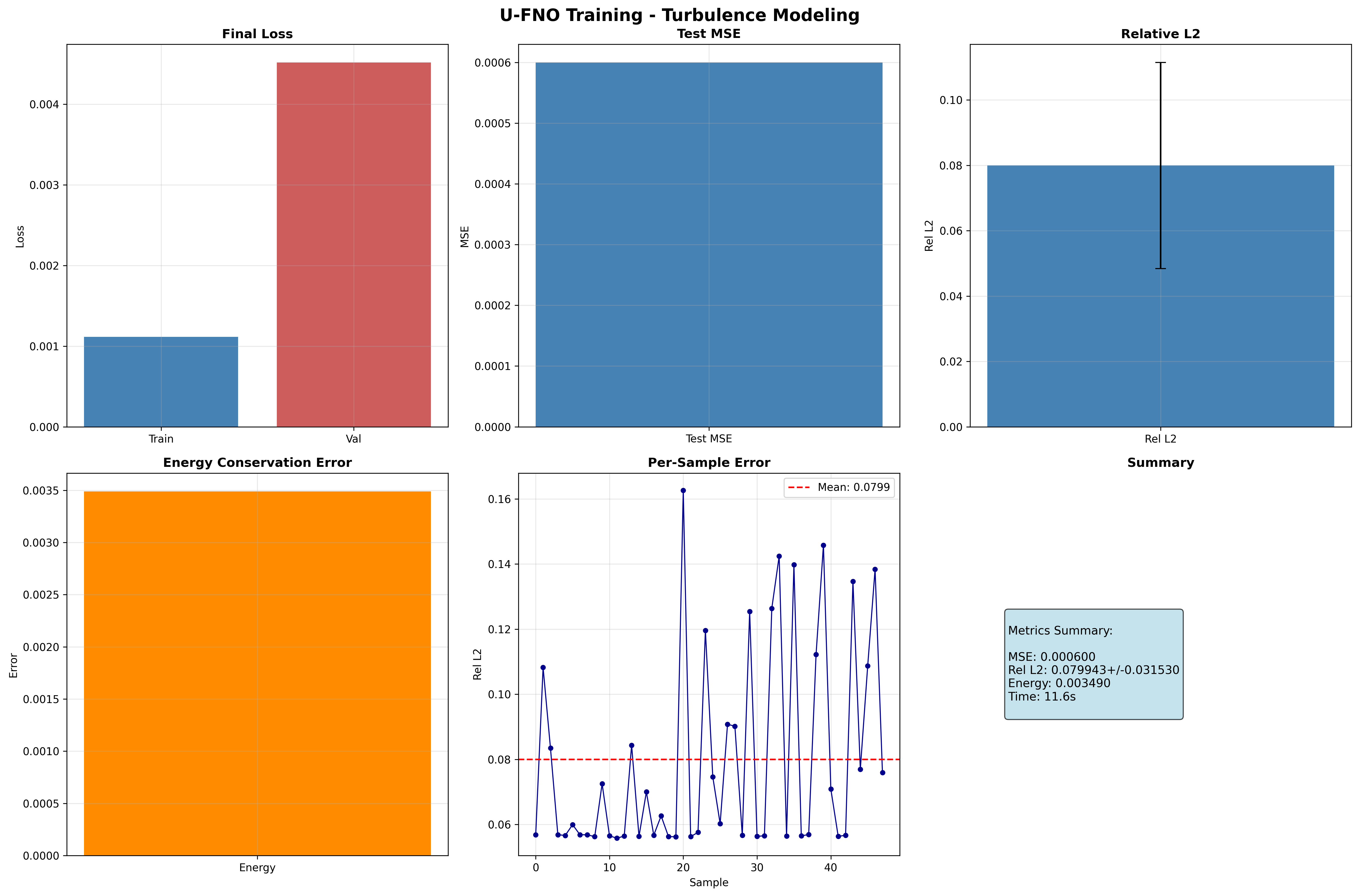
- Training curves: Final loss, MSE, relative L2, energy conservation, and per-sample error
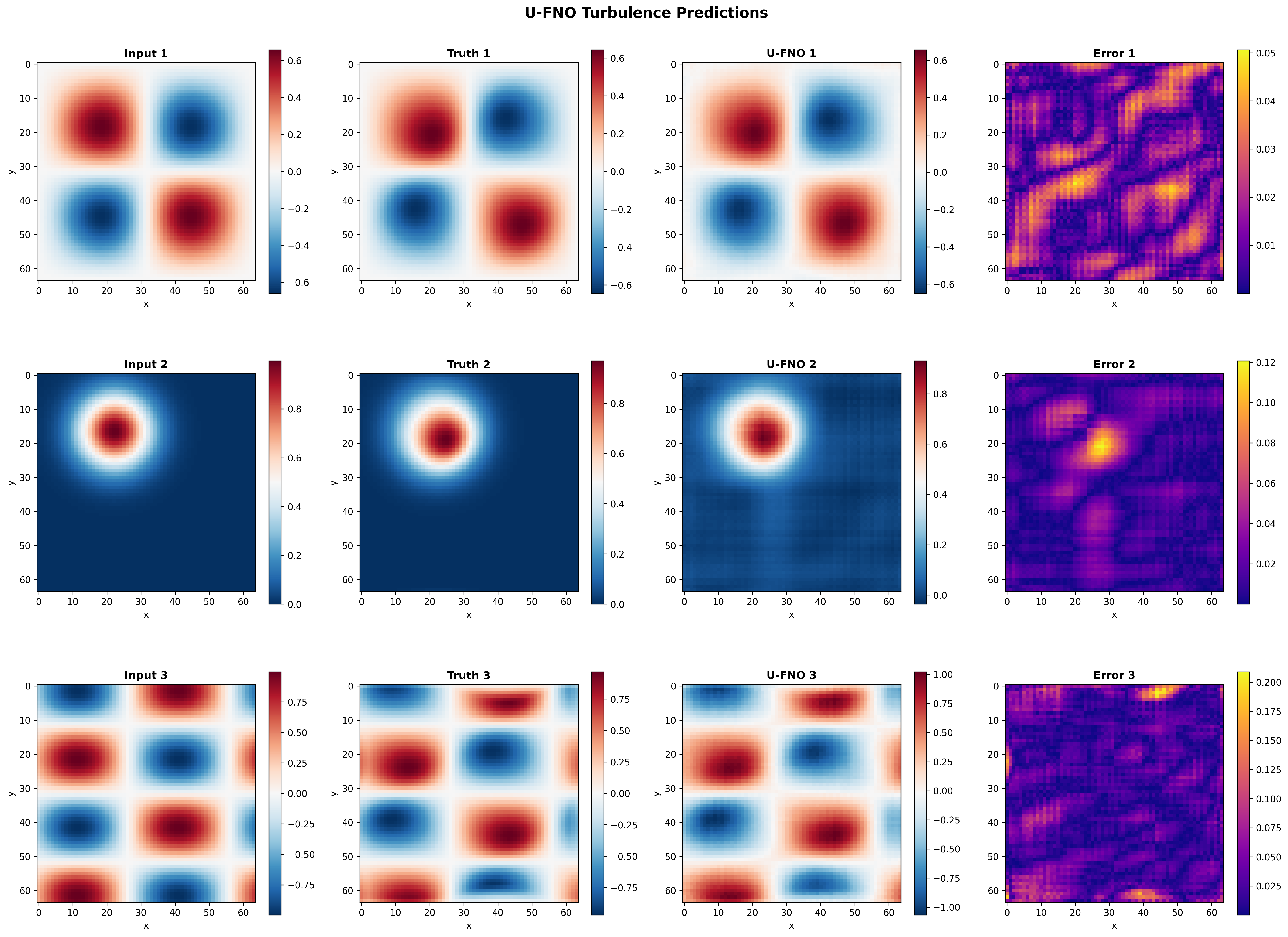
- Sample predictions: Initial velocity magnitude, ground-truth final, U-FNO final, and absolute error (all on \(|v| = \sqrt{u^2 + v^2}\))
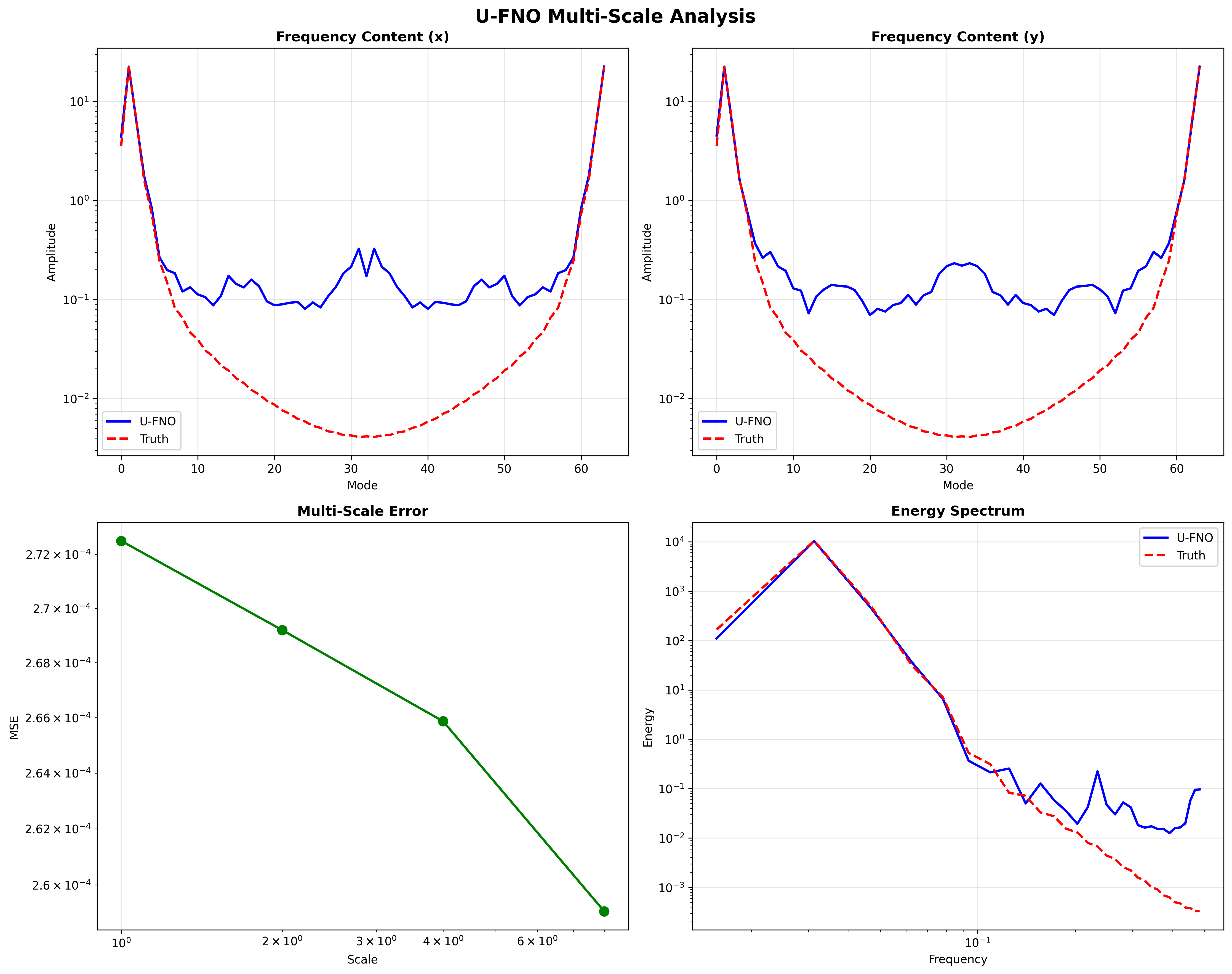
- Multi-scale analysis: Frequency content and energy spectrum of the velocity-magnitude field
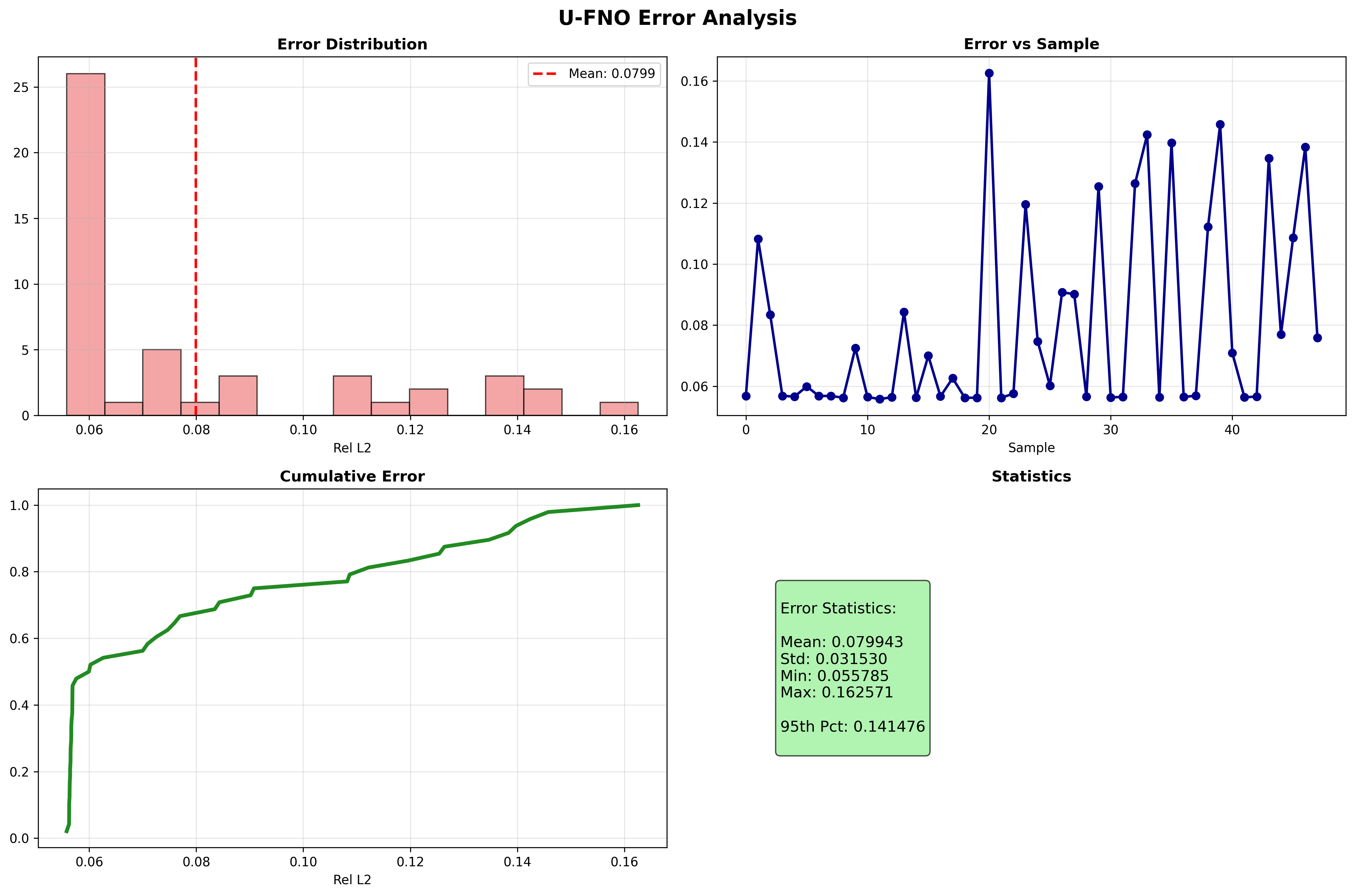
- Error analysis: Error distribution, per-sample error, cumulative distribution, and statistics
Training Curves
Sample Predictions
Multi-Scale Analysis
Error Analysis
Results Summary
Terminal Output:
======================================================================
Full U-FNO Navier-Stokes turbulence example completed in 11.5s
Mean Relative L2 Error: 0.056688
Results saved to: docs/assets/examples/ufno_turbulence
======================================================================
| Metric | Value | Notes |
|---|---|---|
| Test MSE | 0.000166 | Mean squared error on test set |
| Test Relative L2 | 0.056688 ± 0.063488 | Mean ± std relative L2 error |
| Energy Conservation | 0.003750 | Mean energy deviation (lower is better) |
| Final Train Loss | 0.000789 | Training loss at epoch 5 |
| Final Val Loss | 0.001596 | Validation loss at epoch 5 |
| Model Parameters | 240,130,562 | Total trainable parameters |
| Training Time | 11.5s | On GPU (CudaDevice) |
| Resolution | 64x64 | Spatial grid resolution |
What We Achieved
- Built a U-FNO with
GridEmbedding2Dpositional encoding andcreate_turbulence_ufnofactory - Mapped initial velocity \((u, v)\) to final-time velocity for 2D Navier-Stokes turbulence
- Trained with custom energy conservation loss via
trainer.custom_losses["energy"]API - Achieved ~5.7% relative L2 error with only 5 epochs on 304 training samples
- Energy conservation error of 0.003750, showing the physics loss effectively constrains predictions
- Generated multi-scale spectral analysis comparing U-FNO frequency content to ground truth
Interpretation
The U-FNO captures turbulent dynamics effectively even with minimal training. The relative L2 error of ~0.057 with just 5 epochs demonstrates the architecture's efficiency for multi-scale problems. The low energy conservation error (0.003750) confirms that the custom physics loss successfully constrains the model to preserve kinetic energy. The spectral analysis of the velocity-magnitude field shows good agreement between predicted and ground-truth frequency content, with the U-FNO accurately capturing both low-frequency structure and higher-frequency turbulent features.
Next Steps
Experiments to Try
- Longer training: Increase
num_epochsto 50-100 for substantially improved accuracy - Stronger physics loss: Increase the energy loss weight from 0.1 to 0.5 or add vorticity preservation
- Higher resolution: Use
resolution=128orresolution=256for finer turbulent structures - Lower viscosity: Set
viscosity_range=(0.0001, 0.001)for more chaotic turbulent regimes - Compare with standard FNO: Run the same Navier-Stokes problem with
FourierNeuralOperatorto see the U-Net advantage
Related Examples
| Example | Level | What You'll Learn |
|---|---|---|
| FNO Darcy Full | Intermediate | Standard FNO with grid embedding for steady-state problems |
| SFNO Climate Full | Advanced | Conservation-aware training with ConservationConfig on spherical domains |
| SFNO Climate Simple | Intermediate | Minimal SFNO example for quick start |
| UNO Darcy Framework | Intermediate | U-shaped neural operator with zero-shot super-resolution |
| Grid Embeddings | Beginner | Spatial coordinate injection for neural operators |
| Neural Operator Benchmark | Advanced | Cross-architecture performance comparison |
API Reference
create_turbulence_ufno- U-FNO factory for turbulence modelingGridEmbedding2D- 2D spatial coordinate embedding layerTrainer- Training orchestration with custom loss supportTrainingConfig- Training hyperparameter configurationcreate_navier_stokes_loader- datarax-based 2D Navier-Stokes turbulence data loader
Troubleshooting
OOM during training at 64x64 or higher
Symptom: jaxlib.xla_extension.XlaRuntimeError: RESOURCE_EXHAUSTED
Cause: U-FNO has higher memory requirements than standard FNO due to the multi-scale encoder-decoder architecture.
Solution:
# Reduce batch size
config = TrainingConfig(batch_size=8, ...)  # Was 16

# Or enable gradient checkpointing
config = TrainingConfig(gradient_checkpointing=True, gradient_checkpoint_policy="dots_saveable")
NaN in training loss
Symptom: Loss becomes nan after a few epochs.
Cause: Learning rate too high or energy loss producing unstable gradients.
Solution:
# Reduce learning rate
learning_rate = 1e-4  # Was 1e-3

# Or reduce energy loss weight
def energy_loss_fn(model, x, y_pred, y_true):
    pred_energy = jnp.mean(y_pred**2, axis=(2, 3))
    target_energy = jnp.mean(y_true**2, axis=(2, 3))
    return 0.01 * jnp.mean(jnp.abs(pred_energy - target_energy))  # Was 0.1
Grid embedding layout mismatch
Symptom: ValueError about incompatible shapes when applying GridEmbedding2D.
Cause: GridEmbedding2D expects channels-last (B, H, W, C) while U-FNO uses
channels-first (B, C, H, W).
Solution: Convert layouts before and after embedding: