FNO on 2D Navier-Stokes
| Metadata | Value |
|---|---|
| Level | Intermediate |
| Runtime | ~3 min (CPU) / ~30 sec (GPU) |
| Prerequisites | JAX, Flax NNX, FNO basics, CFD concepts |
| Format | Python + Jupyter |
| Memory | ~3 GB RAM |
Overview
This example trains a Fourier Neural Operator (FNO) to learn the solution operator for the 2D incompressible Navier-Stokes equations:
where \(\mathbf{u} = (u, v)\) is the velocity field, \(p\) is pressure, \(\rho\) is density, and \(\nu\) is the kinematic viscosity. The operator we learn maps the initial velocity field to the velocity field at the final time, with the flow parameterized by viscosity. The input and output are both two-channel fields holding the \((u, v)\) velocity components.
What You'll Learn
- Apply the FNO as an initial-condition → final-state solution operator (CFD setting)
- Build incompressible initial conditions from a Taylor-Green vortex
- Train across different kinematic-viscosity regimes
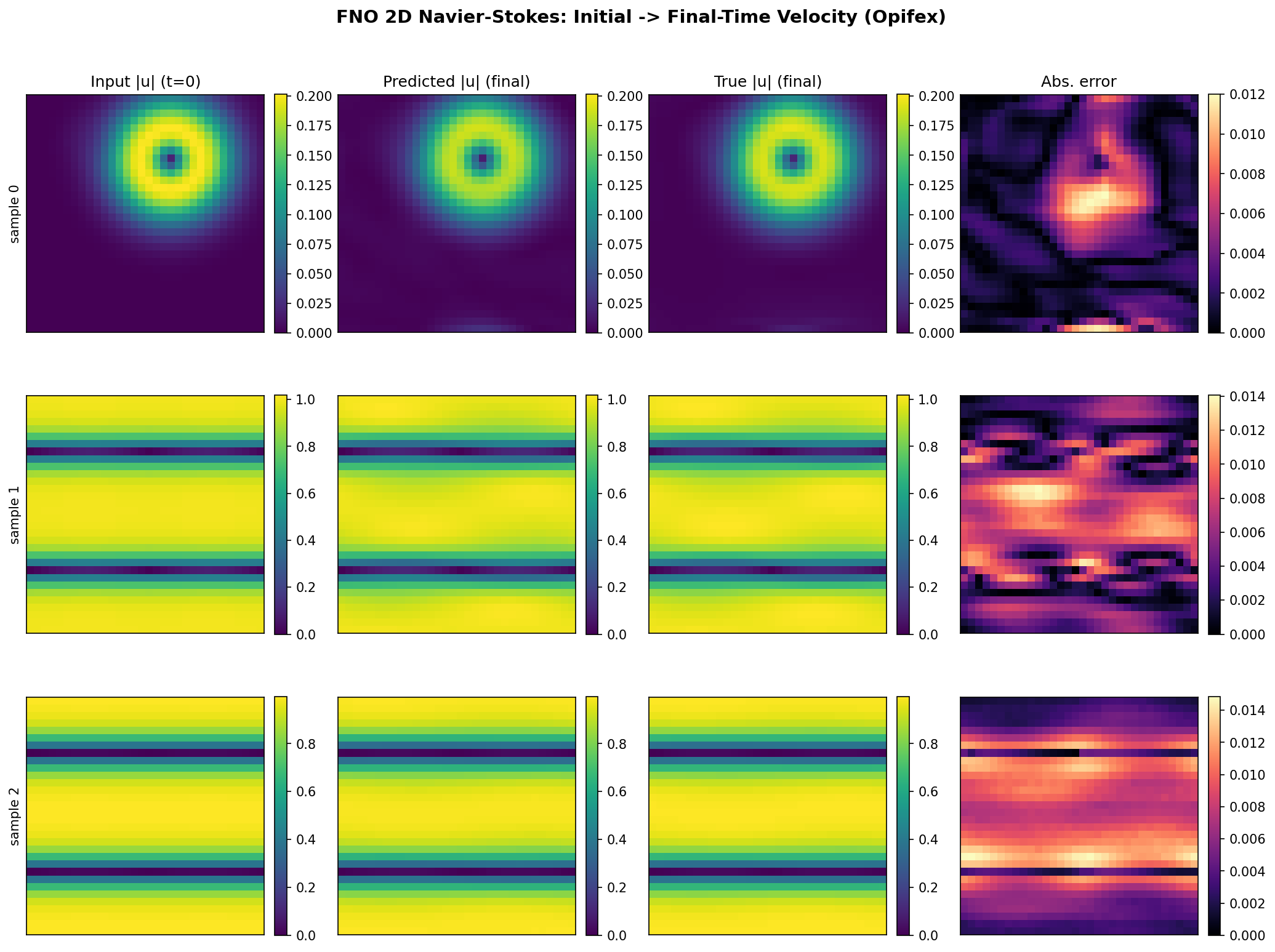
- Evaluate final-time prediction accuracy (MSE / relative L2) and visualise velocity magnitude fields
Files
- Python Script:
examples/neural-operators/fno_navier_stokes.py - Jupyter Notebook:
examples/neural-operators/fno_navier_stokes.ipynb
Quick Start
Key Concepts
The example reuses Opifex's Navier-Stokes data via create_navier_stokes_loader, which
returns a frozen PDELoaders object whose .train/.val pipelines yield channels-first
(b, 2, H, W) batches — the two channels are the \((u, v)\) velocity components. The operator
maps the initial velocity field to the final-time velocity field. Compared with the scalar
FNO on Darcy Flow example, the key differences are the multi-channel
input/output and the time-evolution structure of the target.
from opifex.data.loaders import create_navier_stokes_loader
from opifex.neural.operators.fno.base import FourierNeuralOperator
The data is generated via datarax under the uniform conditioning → final-time contract.
Each batch is a dict with "input" (initial velocity) and "output" (final-time velocity):
n_samples = n_train + n_test
loaders = create_navier_stokes_loader(
    n_samples=n_samples,
    batch_size=batch_size,
    resolution=resolution,
    viscosity_range=(0.001, 0.01),
    time_range=time_range,
    val_fraction=n_test / n_samples,
    seed=seed,
)


def _collect(pipeline):
    """Materialize a datarax pipeline into (inputs, outputs) numpy arrays."""
    inputs, outputs = [], []
    for batch in pipeline:
        inputs.append(np.asarray(batch["input"]))
        outputs.append(np.asarray(batch["output"]))
    return np.concatenate(inputs, axis=0), np.concatenate(outputs, axis=0)


x_train, y_train = _collect(loaders.train)
x_test, y_test = _collect(loaders.val)
The model uses two input channels and two output channels — both velocity fields:
model = FourierNeuralOperator(
    in_channels=2,   # (u, v) initial velocity components
    out_channels=2,  # (u, v) final-time velocity components
    hidden_channels=hidden_width,
    modes=modes,
    num_layers=num_layers,
    rngs=nnx.Rngs(seed),
)
The loss is a plain MSE on the final-time velocity field — no trajectory reshape:
def loss_fn(model, x, y):
    """MSE loss for final-time velocity field prediction."""
    y_pred = model(x)  # (batch, 2, res, res)
    return jnp.mean((y_pred - y) ** 2)
Evaluation reports the test MSE, the mean per-sample relative L2 error, and per-component \((u, v)\) MSE:
predictions = model(x_test_jnp)  # (batch, 2, res, res)
test_mse = float(jnp.mean((predictions - y_test_jnp) ** 2))

pred_flat = predictions.reshape(predictions.shape[0], -1)
true_flat = y_test_jnp.reshape(y_test_jnp.shape[0], -1)
rel_l2 = jnp.linalg.norm(pred_flat - true_flat, axis=1) / jnp.linalg.norm(true_flat, axis=1)
mean_rel_l2 = float(jnp.mean(rel_l2))

u_mse = float(jnp.mean((predictions[:, 0] - y_test_jnp[:, 0]) ** 2))
v_mse = float(jnp.mean((predictions[:, 1] - y_test_jnp[:, 1]) ** 2))
Expected Output
Generating Navier-Stokes data via datarax...
  (Using Taylor-Green vortex initial conditions)
Training: X=(104, 2, 32, 32), Y=(104, 2, 32, 32)
Test:     X=(32, 2, 32, 32), Y=(32, 2, 32, 32)
  X = (batch, 2=[u,v], res, res) = initial velocity
  Y = (batch, 2=[u,v], res, res) = velocity at final time

Creating FNO model...
Model parameters: 2,368,098

Setting up training...
Starting training...

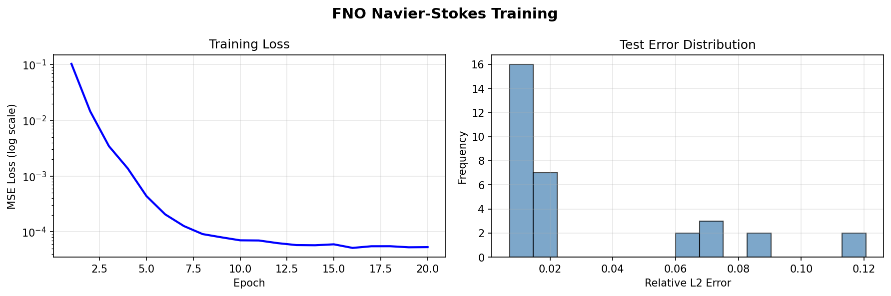
Epoch   1/20: Loss = 0.103224
Epoch   5/20: Loss = 0.000439
Epoch  10/20: Loss = 0.000070
Epoch  15/20: Loss = 0.000060
Epoch  20/20: Loss = 0.000053

Training completed in 2.2s

Running evaluation...
Test MSE:         0.000061
Test Relative L2: 0.031566

Per-component final-time MSE:
  u-MSE=0.000073, v-MSE=0.000048
The FNO reaches a relative L2 error of about 0.032 (≈3.2%) on the held-out test set, with a test MSE of \(6.1\times10^{-5}\) and per-component MSE of \(7.3\times10^{-5}\) (\(u\)) and \(4.8\times10^{-5}\) (\(v\)), training in roughly two seconds on a GPU.
Results
Next Steps
- FNO on Burgers Equation — another time-dependent operator-learning task
- U-FNO on Turbulence — U-shaped FNO for turbulent flows
FourierNeuralOperator— FNO model class