FNO on Darcy Flow

Metadata	Value
Level	Intermediate
Runtime	~3 min (CPU) / ~1 min (GPU)
Prerequisites	JAX, Flax NNX, Neural Operators basics
Format	Python + Jupyter
Memory	~2 GB RAM

Overview

This tutorial demonstrates training a Fourier Neural Operator (FNO) on the Darcy flow problem, a standard benchmark in neural operator research. The Darcy flow equation models steady-state fluid flow through porous media, mapping a permeability coefficient field to a pressure solution field.

What makes this example stand out is the composition of GridEmbedding2D with FourierNeuralOperator. Grid embeddings inject spatial coordinate information as additional input channels, giving the FNO positional awareness that improves operator learning for spatially varying problems. The example uses Opifex's own Darcy data via create_darcy_loader (smooth Darcy, solved with the accurate direct solver) and the standard operator-learning recipe: Gaussian normalization, the relative-L2 loss, AdamW with weight decay, and an exponential learning-rate schedule. It covers the full pipeline: loading the data, model creation, training with the unified Trainer API, evaluation with L2 relative error, and full visualization of predictions and error distributions.

This is the FNO counterpart to UNO on Darcy Flow and Your First Neural Operator, which use the same synthetic Darcy data and recipe.

What You'll Learn

1. Compose GridEmbedding2D with FourierNeuralOperator for positional encoding
2. Load Darcy flow data with create_darcy_loader (datarax pipelines)
3. Apply Gaussian normalization and the relative-L2 loss via LossConfig
4. Use AdamW, weight decay, and an exponential learning-rate schedule
5. Evaluate with L2 relative error and a train-vs-test overfitting check
6. Visualize predictions, ground truth comparisons, and error distributions

Coming from NeuralOperator (PyTorch)?

If you are familiar with the neuraloperator library, here is how Opifex compares for this workflow:

NeuralOperator (PyTorch)	Opifex (JAX)
FNO(n_modes, hidden_channels)	FourierNeuralOperator(modes=, hidden_channels=, num_layers=, rngs=)
Manual torch.meshgrid for positional encoding	GridEmbedding2D(in_channels=, grid_boundaries=)
Custom Darcy dataset / loader	create_darcy_loader(n_samples=, resolution=, ...)
LpLoss(d=2, p=2) (relative)	LossConfig(loss_type="relative_l2")
trainer.train(train_loader, epochs)	Trainer(model, config, rngs).fit(train_data, val_data)
AdamW(lr, weight_decay) + LR schedule	OptimizationConfig(optimizer="adamw", weight_decay=, schedule_type=...)
Manual training loop with loss.backward()	Automatic JIT-compiled training loop via Trainer.fit()

Key differences:

1. Explicit PRNG: Opifex uses JAX's explicit rngs=nnx.Rngs(42) instead of global random state
2. Composable grid embedding: GridEmbedding2D composes cleanly with FourierNeuralOperator via standard nnx.Module subclassing
3. XLA compilation: Automatic JIT compilation in Trainer.fit() for faster training
4. Functional transforms: jax.grad, jax.vmap, jax.pmap for composable differentiation and parallelism

Files

• Python Script: examples/neural-operators/fno_darcy.py
• Jupyter Notebook: examples/neural-operators/fno_darcy.ipynb

Quick Start

Run the Python Script

source activate.sh && python examples/neural-operators/fno_darcy.py

Run the Jupyter Notebook

jupyter lab examples/neural-operators/fno_darcy.ipynb

Core Concepts

The Fourier Neural Operator

The FNO learns operator mappings between function spaces by parameterizing convolution kernels in Fourier space. Each spectral layer performs four operations:

1. FFT: Transform input to the frequency domain
2. Spectral convolution: Apply learned linear transform to truncated Fourier modes
3. Inverse FFT: Transform back to the spatial domain
4. Skip connection: Add a local linear transform (pointwise convolution)

This spectral approach gives each layer a global receptive field, enabling the FNO to capture long-range spatial correlations in a single pass.

FNO Architecture with Grid Embedding

In this example, we compose GridEmbedding2D with FourierNeuralOperator to inject spatial coordinate information before the spectral layers process the data. The grid embedding appends x and y coordinate channels to the input, expanding a 1-channel permeability field into a 3-channel tensor (permeability + x-coord + y-coord).

graph LR
    subgraph Input
        A["Permeability Field<br/>a(x) : R^(1x32x32)"]
    end

    subgraph Embedding["Grid Embedding"]
        B["GridEmbedding2D<br/>Append (x, y) coords<br/>1 ch -> 3 ch"]
    end

    subgraph FNO["Fourier Neural Operator"]
        C["Lifting Layer<br/>P: R^3 -> R^32"]
        D["Spectral Layer 1<br/>FFT -> Conv -> IFFT + Skip"]
        E["Spectral Layer 2<br/>FFT -> Conv -> IFFT + Skip"]
        F["Spectral Layer 3<br/>FFT -> Conv -> IFFT + Skip"]
        G["Spectral Layer 4<br/>FFT -> Conv -> IFFT + Skip"]
        H["Projection Layer<br/>Q: R^32 -> R^1"]
    end

    subgraph Output
        I["Pressure Field<br/>u(x) : R^(1x32x32)"]
    end

    A --> B --> C --> D --> E --> F --> G --> H --> I

    style A fill:#e3f2fd,stroke:#1976d2
    style B fill:#fff3e0,stroke:#f57c00
    style I fill:#c8e6c9,stroke:#388e3c

Darcy Flow Problem

The Darcy flow equation models steady-state fluid flow through porous media:

\[-\nabla \cdot (a(x) \nabla u(x)) = f(x), \quad x \in D\]

Variable	Meaning	Role
\(a(x)\)	Permeability field	Input function (what we observe)
\(u(x)\)	Pressure field	Output function (what we predict)
\(f(x)\)	Forcing term	Fixed (constant source)
\(D\)	Domain	Unit square \([0, 1]^2\)

The neural operator learns the mapping \(a(x) \mapsto u(x)\) from data, without needing to solve the PDE at inference time.

Implementation

Step 1: Imports and Setup

import time
import warnings
from pathlib import Path

warnings.filterwarnings("ignore")

import jax
import jax.numpy as jnp
import matplotlib as mpl
import numpy as np
from flax import nnx

mpl.use("Agg")
import matplotlib.pyplot as plt

# Opifex framework imports
from opifex.core.training import Trainer, TrainingConfig
from opifex.core.training.config import LossConfig, OptimizationConfig
from opifex.data.loaders import create_darcy_loader
from opifex.neural.operators.common.embeddings import GridEmbedding2D
from opifex.neural.operators.fno.base import FourierNeuralOperator

Terminal Output:

======================================================================
Opifex Example: FNO on Darcy Flow
======================================================================
JAX backend: gpu
JAX devices: [CudaDevice(id=0)]

Step 2: Configuration

Define the hyperparameters for data generation, model architecture, and training:

RESOLUTION = 32  # synthetic Darcy resolution
N_TRAIN = 1000
N_TEST = 100
BATCH_SIZE = 32
NUM_EPOCHS = 200
LEARNING_RATE = 5e-3  # AdamW initial LR
WEIGHT_DECAY = 1e-4  # regularization to combat overfitting
MODES = 12
HIDDEN_WIDTH = 32
NUM_LAYERS = 4
DOMAIN_PADDING = 0.25  # fraction of each spatial dim (resolution-invariant Gibbs padding)
SEED = 42

OUTPUT_DIR = Path("docs/assets/examples/fno_darcy")
OUTPUT_DIR.mkdir(parents=True, exist_ok=True)

Terminal Output:

Resolution: 32x32
Training samples: 1000, Test samples: 100
Batch size: 32, Epochs: 200
FNO config: modes=12, width=32, layers=4
Optimizer: AdamW (lr=0.005, weight_decay=0.0001)
LR schedule: exponential, x0.5 every 60 epochs

Hyperparameter	Value	Purpose
RESOLUTION	32	Spatial grid resolution (32x32)
N_TRAIN / N_TEST	1000 / 100	Train / test split from create_darcy_loader
BATCH_SIZE	32	Samples per training batch
NUM_EPOCHS	200	Training iterations over full dataset
LEARNING_RATE	5e-3	AdamW initial learning rate
WEIGHT_DECAY	1e-4	L2 weight decay (regularization)
MODES	12	Number of Fourier modes retained per dimension
HIDDEN_WIDTH	32	Width of the spectral layers
DOMAIN_PADDING	0.25	Spatial padding fraction (resolution-invariant) to reduce the Gibbs phenomenon

Step 3: Data Loading

We generate Darcy flow data with create_darcy_loader (smooth Darcy, solved with the accurate direct solver) and serve it via datarax pipelines. create_darcy_loader returns a frozen PDELoaders with .train / .val datarax pipelines, split by val_fraction. The batches are already channels-first {"input": (b, 1, H, W), "output": (b, 1, H, W)}, so we just drain each pipeline into arrays for Trainer.fit().

loaders = create_darcy_loader(
    n_samples=n_samples,
    batch_size=batch_size,
    resolution=resolution,
    val_fraction=n_test / n_samples,
    seed=seed,
)

# Collect the datarax pipelines into arrays for Trainer.fit(). Batches are
# channels-first {"input": (b, 1, H, W), "output": (b, 1, H, W)}.
def _collect(pipeline) -> tuple[np.ndarray, np.ndarray]:
    inputs, outputs = [], []
    for batch in pipeline:
        inputs.append(np.asarray(batch["input"]))
        outputs.append(np.asarray(batch["output"]))
    return np.concatenate(inputs, axis=0), np.concatenate(outputs, axis=0)

x_train, y_train = _collect(loaders.train)
x_test, y_test = _collect(loaders.val)

Terminal Output:

Generating Darcy flow data (jit+vmap) and serving via datarax...
Training data: X=(1024, 1, 32, 32), Y=(1024, 1, 32, 32)
Test data:     X=(128, 1, 32, 32), Y=(128, 1, 32, 32)

We fit Gaussian statistics on the training set, normalize all splits, and un-normalize predictions before measuring the physical-space relative L2 error:

x_mean, x_std = x_train.mean(), x_train.std()
y_mean, y_std = y_train.mean(), y_train.std()

x_train_n = (x_train - x_mean) / x_std
y_train_n = (y_train - y_mean) / y_std

Terminal Output:

Input mean/std:  0.1778 / 0.1302
Output mean/std: 0.213690 / 0.155666

Step 4: Model Creation -- Composing GridEmbedding2D with FNO

The key architectural pattern in this example is composing GridEmbedding2D with FourierNeuralOperator inside a single nnx.Module. The grid embedding appends spatial coordinates as additional channels, providing the FNO with positional awareness.

class FNOWithEmbedding(nnx.Module):
    """FNO model with built-in grid embedding for positional encoding."""

    def __init__(
        self,
        in_channels: int,
        out_channels: int,
        modes: int,
        hidden_channels: int,
        num_layers: int,
        grid_boundaries: list[list[float]],
        *,
        domain_padding: float,
        rngs: nnx.Rngs,
    ) -> None:
        super().__init__()
        self.grid_embedding = GridEmbedding2D(
            in_channels=in_channels,
            grid_boundaries=grid_boundaries,
        )
        self.fno = FourierNeuralOperator(
            in_channels=self.grid_embedding.out_channels,
            out_channels=out_channels,
            hidden_channels=hidden_channels,
            modes=modes,
            num_layers=num_layers,
            domain_padding=domain_padding,
            rngs=rngs,
        )

    def __call__(self, x: jax.Array) -> jax.Array:
        """Forward pass: grid embedding -> FNO."""
        # Convert (batch, channels, H, W) -> (batch, H, W, channels) for embedding
        x_hwc = jnp.moveaxis(x, 1, -1)
        x_embedded = self.grid_embedding(x_hwc)
        # Convert back to (batch, channels, H, W) for FNO
        x_chw = jnp.moveaxis(x_embedded, -1, 1)
        return self.fno(x_chw)

Create the model instance:

model = FNOWithEmbedding(
    in_channels=1,
    out_channels=1,
    modes=MODES,
    hidden_channels=HIDDEN_WIDTH,
    num_layers=NUM_LAYERS,
    grid_boundaries=[[0.0, 1.0], [0.0, 1.0]],
    domain_padding=DOMAIN_PADDING,
    rngs=nnx.Rngs(SEED),
)

Terminal Output:

Creating FNO model with grid embedding...
Model: FNO + GridEmbedding2D
  Input channels: 1 (+ 2 grid coords = 3 after embedding)
  Fourier modes: 12, Hidden width: 32, Layers: 4
  Total parameters: 2,368,001

Why Grid Embeddings?

GridEmbedding2D appends normalized x and y coordinates to each spatial location, expanding the input from 1 channel to 3 channels. This positional encoding helps the FNO learn spatially varying operators where the solution depends on position within the domain, not just the local input value.

Step 5: The Relative-L2 Loss and Training

We train with the relative-L2 loss, the standard operator-learning objective. It normalizes each sample's L2 error by the L2 norm of the target, so every example contributes proportionally regardless of its magnitude:

\[ \mathcal{L}_{L2} = \frac{\|u_p - u\|_2}{\|u\|_2} \]

The loss is selected declaratively via LossConfig — no Trainer subclass is needed. Training uses AdamW, weight decay, and an exponential learning-rate schedule (halve every 60 epochs), all via OptimizationConfig:

config = TrainingConfig(
    num_epochs=NUM_EPOCHS,
    batch_size=BATCH_SIZE,
    validation_frequency=20,
    verbose=True,
    loss_config=LossConfig(loss_type="relative_l2"),
    optimization_config=OptimizationConfig(
        optimizer="adamw",
        learning_rate=LEARNING_RATE,
        weight_decay=WEIGHT_DECAY,
        schedule_type="exponential",
        transition_steps=LR_TRANSITION_STEPS,
        decay_rate=LR_DECAY_RATE,
    ),
)

trainer = Trainer(model=model, config=config, rngs=nnx.Rngs(SEED))

trained_model, metrics = trainer.fit(
    train_data=(jnp.array(X_train_n), jnp.array(Y_train_n)),
    val_data=(jnp.array(X_test_n), jnp.array(Y_test_n)),
)

Terminal Output:

Setting up Trainer...
Optimizer: AdamW (lr=0.005, weight_decay=0.0001)
Loss: relative L2 (the standard operator-learning objective)

Starting training...
Training completed in 18.4s
Final train loss: 0.006624664645642042
Final val loss:   0.0001833601709222421

Step 6: Full Evaluation

Predictions are un-normalized back to physical pressure units before measuring the error. We run both the test and training sets through the model in batches (to bound memory) and compare their relative L2 errors to expose any overfitting:

# Un-normalize predictions back to physical pressure units
predictions = predict_in_batches(trained_model, x_test_jnp) * y_std + y_mean
train_predictions = predict_in_batches(trained_model, x_train_jnp) * y_std + y_mean

# Test relative L2 (per sample) in physical units
test_mse = float(jnp.mean((predictions - y_test_jnp) ** 2))
per_sample_rel_l2 = per_sample_relative_l2(predictions, y_test_jnp)
mean_rel_l2 = float(jnp.mean(per_sample_rel_l2))
train_rel_l2 = float(relative_l2_error(train_predictions, y_train_jnp))

Terminal Output:

Running evaluation...
Train Relative L2: 0.004973
Test  Relative L2: 0.007588
Overfitting gap (test - train): +0.002615
Test MSE:         4.024144e-06
Min Relative L2:  0.004003
Max Relative L2:  0.021948

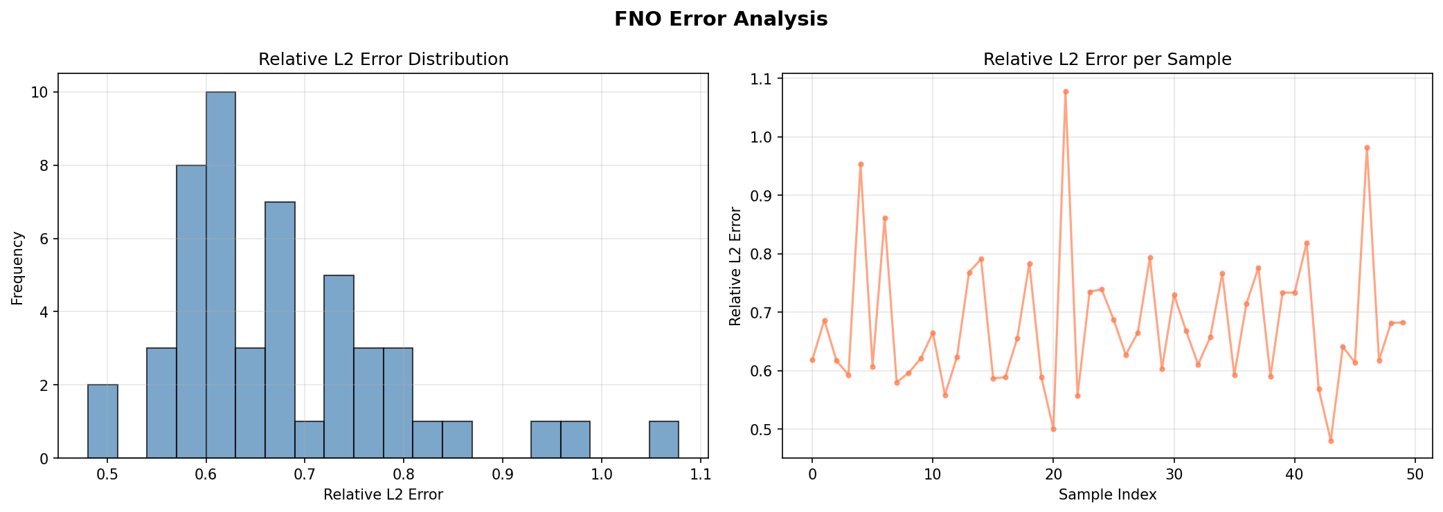
Reading the Relative L2 Error

Errors are measured in physical pressure units after un-normalizing the predictions. A test relative L2 of ~0.76% with a sub-0.3% train-vs-test gap confirms the FNO learns the Darcy operator accurately and generalizes well on this data.

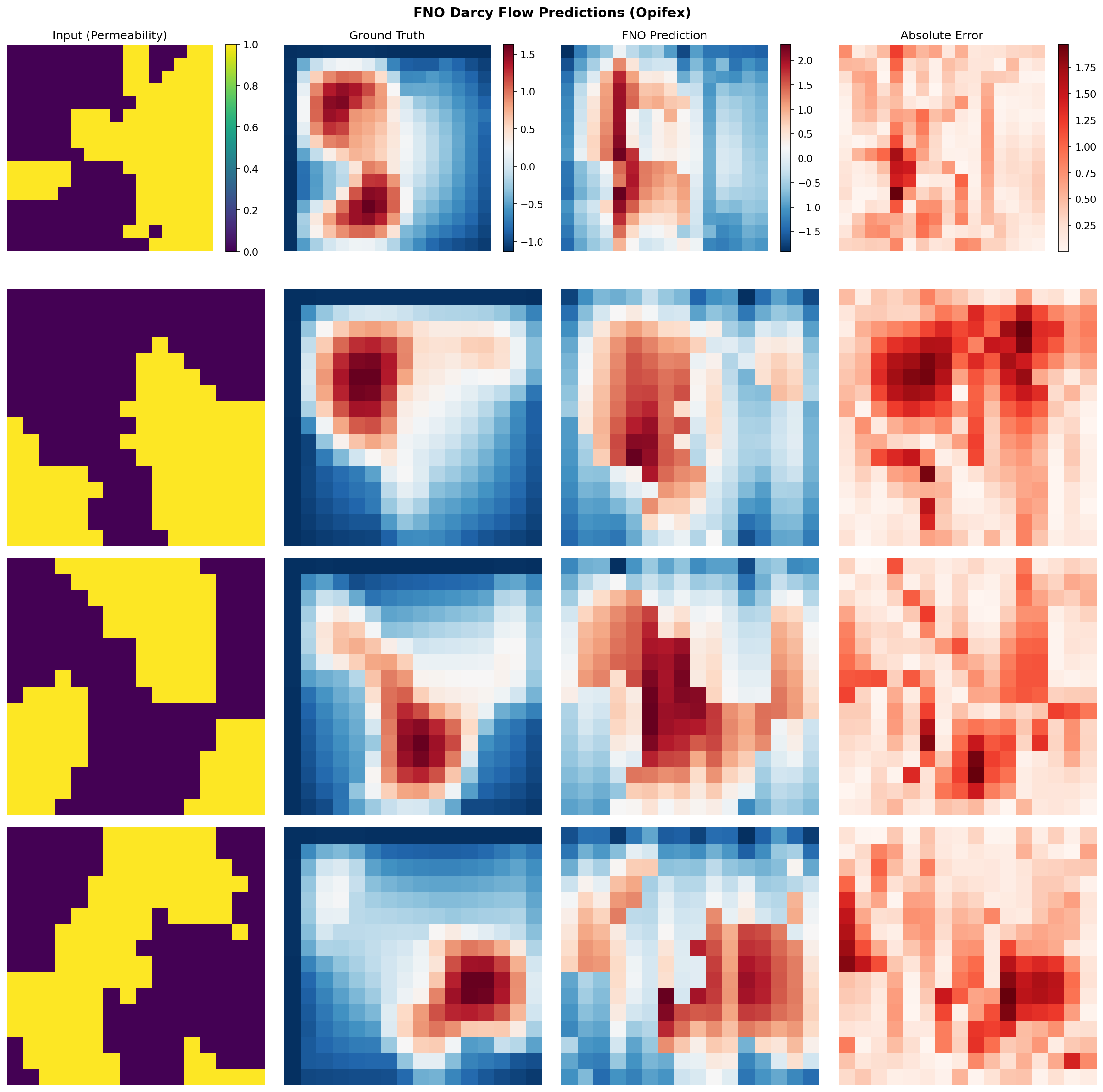
Step 7: Visualization

Generate full visualizations including sample predictions, error maps, and error distribution analysis.

n_vis = min(4, len(x_test))
fig, axes = plt.subplots(n_vis, 4, figsize=(16, 4 * n_vis))
fig.suptitle(
    "FNO Darcy Flow Predictions (Opifex)", fontsize=14, fontweight="bold"
)

for i in range(n_vis):
    axes[i, 0].imshow(x_test[i, 0], cmap="viridis")    # Input (permeability)
    axes[i, 1].imshow(y_test[i, 0], cmap="RdBu_r")     # Ground truth
    axes[i, 2].imshow(pred_np, cmap="RdBu_r")           # FNO prediction
    error = np.abs(pred_np - y_test[i, 0])
    axes[i, 3].imshow(error, cmap="Reds")               # Absolute error

plt.savefig(OUTPUT_DIR / "sample_predictions.png", dpi=150, bbox_inches="tight")

Terminal Output:

Generating visualizations...
Sample predictions saved to docs/assets/examples/fno_darcy/sample_predictions.png
Error analysis saved to docs/assets/examples/fno_darcy/error_analysis.png

Sample Predictions

Error Analysis

Results Summary

Terminal Output:

======================================================================
FNO Darcy Flow example completed in 18.4s
Test MSE: 4.024144e-06, Relative L2: 0.007588
Results saved to: docs/assets/examples/fno_darcy
======================================================================

Metric	Value	Notes
Train Relative L2	0.004973	Mean relative L2 on the training set (physical units)
Test Relative L2	0.007588	Mean relative L2 on the test set (physical units)
Min Relative L2	0.004003	Best per-sample test relative L2
Max Relative L2	0.021948	Worst per-sample test relative L2
Test MSE	4.02e-06	Mean squared error on the test set
Final Train Loss	6.62e-3	Relative-L2 training loss at epoch 200
Final Val Loss	1.83e-4	Relative-L2 validation loss at epoch 200
Training Time	18.4s	On GPU (CudaDevice)
Total Parameters	2,368,001	FNO + GridEmbedding2D

What We Achieved

• Composed GridEmbedding2D with FourierNeuralOperator in a clean nnx.Module subclass
• Trained on Opifex's synthetic Darcy data with the relative-L2 loss, AdamW + weight decay, and an exponential learning-rate schedule via Trainer.fit()
• Evaluated with per-sample L2 relative error and an explicit train-vs-test overfitting check
• Generated prediction comparison and error distribution visualizations

Interpretation

This example demonstrates the full Opifex neural operator workflow on Opifex's own Darcy data. The FNO reaches a train relative L2 around 0.50% and a test relative L2 around 0.76% in physical pressure units, with a sub-0.3% train-vs-test gap. The relative-L2 loss, weight decay, and LR schedule together drive accurate operator learning without overfitting, consistent with the UNO and Your First Neural Operator examples on the same data.

Next Steps

Experiments to Try

1. Swap the loss: Compare the relative-L2 objective against an H1 (Sobolev) gradient-aware loss to penalize errors in the field gradients as well as the values
2. Tune the schedule: Adjust LR_DECAY_RATE / LR_TRANSITION_STEPS or switch schedule_type to cosine
3. Tune regularization: Increase WEIGHT_DECAY (1e-3 .. 1e-2) to trade train fit for generalization
4. Tune Fourier modes: Try larger MODES or HIDDEN_WIDTH for more capacity
5. Raise the resolution: Generate create_darcy_loader data at 64x64 for a sharper benchmark

Related Examples

Example	Level	What You'll Learn
Grid Embeddings	Beginner	Spatial coordinate injection for neural operators
DISCO Convolutions	Intermediate	Discrete-continuous convolutions for arbitrary grids
UNO on Darcy Flow	Intermediate	Multi-resolution U-shaped neural operator for Darcy flow
SFNO Climate	Intermediate	Spherical FNO for climate modeling on the sphere
U-FNO Turbulence	Intermediate	U-Net enhanced FNO for turbulence problems
Neural Operator Benchmark	Advanced	Cross-architecture comparison (FNO, UNO, SFNO, U-FNO)

API Reference

• FourierNeuralOperator - FNO model class with spectral convolution layers
• GridEmbedding2D - 2D spatial coordinate embedding layer
• Trainer - Unified training orchestration with JIT compilation
• TrainingConfig - Training hyperparameter configuration
• OptimizationConfig - Optimizer, weight decay, and LR-schedule configuration

Troubleshooting

OOM during training

Symptom: jaxlib.xla_extension.XlaRuntimeError: RESOURCE_EXHAUSTED

Cause: Model or batch size exceeds available GPU memory, especially at higher resolutions.

Solution:

# Option 1: Reduce batch size
config = TrainingConfig(batch_size=16, ...)  # Was 32

# Option 2: Enable gradient checkpointing via TrainingConfig
config = TrainingConfig(gradient_checkpointing=True, gradient_checkpoint_policy="dots_saveable")

# Option 3: Use mixed precision
X_train = X_train.astype(jnp.bfloat16)  # 40-50% memory reduction

NaN in training loss

Symptom: Loss becomes nan after a few epochs.

Cause: Learning rate too high or numerical instability in spectral convolutions.

Solution:

# Reduce learning rate and add gradient clipping
import optax

optimizer = optax.chain(
    optax.clip_by_global_norm(1.0),
    optax.adam(1e-4),  # Reduced from 1e-3
)

Shape mismatch after grid embedding

Symptom: ValueError about incompatible shapes when composing GridEmbedding2D with FourierNeuralOperator.

Cause: GridEmbedding2D expects channels-last format (batch, H, W, channels), while FourierNeuralOperator uses channels-first (batch, channels, H, W).

Solution: Use jnp.moveaxis to convert between layouts, as shown in the FNOWithEmbedding class:

def __call__(self, x):
    # channels-first -> channels-last for embedding
    x_hwc = jnp.moveaxis(x, 1, -1)
    x_embedded = self.grid_embedding(x_hwc)
    # channels-last -> channels-first for FNO
    x_chw = jnp.moveaxis(x_embedded, -1, 1)
    return self.fno(x_chw)