Your First PINN: Solving the Poisson Equation¶

Metadata	Value
Level	Beginner
Runtime	~30 seconds (GPU) / ~1 min (CPU)
Prerequisites	Basic Python, calculus
Format	Python + Jupyter
Memory	~500 MB RAM

Overview¶

This tutorial demonstrates Physics-Informed Neural Networks (PINNs) using Opifex's high-level APIs. You'll learn to solve PDEs WITHOUT any training data, using only the governing equation and Opifex's built-in solver infrastructure.

Opifex APIs demonstrated:

Interval: 1D geometry class for computational domains
create_poisson_pinn: Factory function for creating Poisson PINN models
PINNSolver: High-level solver with generic solve() method
poisson_residual: Factory function to create PDE residual (explicit, not hidden)
PINNConfig: Configuration composing with PhysicsLossConfig for loss weights

Problem: Find u(x) satisfying:

PDE: -u''(x) = π² sin(πx) on [-1, 1]
Boundary Conditions: u(-1) = u(1) = 0
Exact Solution: u(x) = sin(πx)

We'll achieve <0.2% L2 relative error in just 2000 iterations (~30 seconds).

What You'll Learn¶

Understand the PINN paradigm: embedding physics into the loss function
Use Interval geometry for 1D domains
Use create_poisson_pinn factory for creating PINN architectures
Use poisson_residual factory to create PDE residual functions
Configure training with PINNConfig (iterations, learning rate, loss weights)
Solve using PINNSolver.solve() with explicit residual functions
Evaluate against the known analytical solution

Coming from DeepXDE?¶

If you're familiar with DeepXDE, here's how Opifex compares:

DeepXDE	Opifex (JAX)
`dde.geometry.Interval(-1, 1)`	`Interval(-1.0, 1.0)`
`dde.nn.FNN([1, 50, 50, 50, 1], "tanh")`	`create_poisson_pinn(spatial_dim=1, hidden_dims=[50,50,50])`
Manual loss weight tuning	`PINNConfig(loss_config=PhysicsLossConfig(...))`
`model.train(iterations=2000)`	`PINNSolver(pinn).solve(geometry, residual_fn, bc_fn)`
`model.compile("adam", lr=1e-3)`	`PINNConfig(learning_rate=1e-3)`
String-based PDE selection	`poisson_residual(source_fn)` — explicit factory

Key differences:

Factory Functions for PDEs: poisson_residual(), heat_residual(), etc. — explicit, type-safe, infinitely extensible
Composition Pattern: PINNConfig composes with PhysicsLossConfig for loss weights
Generic Solve API: solve(geometry, residual_fn, bc_fn) — same method for any PDE
XLA JIT compilation: 2-3x faster training via automatic compilation

Files¶

Python Script: examples/getting-started/first_pinn.py
Jupyter Notebook: examples/getting-started/first_pinn.ipynb

Quick Start¶

Run the Python Script¶

source activate.sh && python examples/getting-started/first_pinn.py

Run the Jupyter Notebook¶

jupyter lab examples/getting-started/first_pinn.ipynb

Core Concepts¶

The PINN Paradigm¶

Traditional neural networks learn from data: given (input, output) pairs, minimize prediction error. PINNs take a fundamentally different approach: they learn from physics.

graph TB
    subgraph Traditional["Traditional ML"]
        A1["Training Data<br/>(x, u) pairs"] --> B1["Neural Network"]
        B1 --> C1["Minimize<br/>||u_pred - u_data||²"]
    end

    subgraph PINN["Physics-Informed NN"]
        A2["Collocation Points<br/>x samples"] --> B2["Neural Network<br/>u_θ(x)"]
        B2 --> C2["Minimize<br/>||PDE Residual||² + ||BC Error||²"]
    end

    style Traditional fill:#fff3e0,stroke:#f57c00
    style PINN fill:#e3f2fd,stroke:#1976d2

The Poisson Equation¶

The 1D Poisson equation is:

\[-\frac{d^2 u}{dx^2} = f(x)\]

With source term f(x) = π² sin(πx) and boundary conditions u(-1) = u(1) = 0, the exact solution is u(x) = sin(πx).

This is the perfect first PINN example because:

Known exact solution — we can measure error precisely
Simple 1D domain — easy to visualize
Linear PDE — stable training dynamics

Opifex PINN Architecture¶

Opifex provides a high-level API that handles all the complexity:

graph LR
    subgraph Input["User Provides"]
        A["Geometry<br/>(Interval)"]
        B["poisson_residual()<br/>factory"]
        C["Boundary values<br/>bc_fn"]
    end

    subgraph Opifex["PINNSolver.solve()"]
        D["AutoDiffEngine<br/>∇²u(x)"]
        E["PhysicsLossComposer<br/>weighted losses"]
        F["Training Loop<br/>Adam optimizer"]
    end

    subgraph Output["Returns"]
        G["PINNResult<br/>model, losses, metrics"]
    end

    A --> F
    B --> D
    C --> E
    D --> E
    E --> F
    F --> G

    style D fill:#e3f2fd,stroke:#1976d2
    style E fill:#e3f2fd,stroke:#1976d2

Implementation¶

Step 1: Imports¶

from pathlib import Path

import jax
import jax.numpy as jnp
import matplotlib as mpl
from flax import nnx

from opifex.geometry import Interval
from opifex.neural.pinns import create_poisson_pinn
from opifex.solvers import PINNConfig, PINNSolver, poisson_residual

Terminal Output:

============================================================
Your First PINN: 1D Poisson Equation (Opifex APIs)
============================================================
JAX backend: gpu

Step 2: Define the Problem¶

def exact_solution(x):
    """Analytical solution: u(x) = sin(pi*x)."""
    return jnp.sin(jnp.pi * x)

def source_term(x):
    """Source term: f(x) = pi^2 * sin(pi*x)."""
    return jnp.pi**2 * jnp.sin(jnp.pi * x)

def boundary_condition(x):
    """Boundary condition: u = 0 at boundaries."""
    return jnp.zeros_like(x[..., 0])

Step 3: Define the Geometry¶

Use Opifex's Interval class for 1D domains:

geometry = Interval(-1.0, 1.0)

Terminal Output:

Defining geometry using Interval...
  Domain: [-1.0, 1.0]
  Length: 2.0

Step 4: Create the PINN Model¶

Use create_poisson_pinn factory to create an appropriate architecture:

pinn = create_poisson_pinn(
    spatial_dim=1,
    hidden_dims=[50, 50, 50],
    rngs=nnx.Rngs(42),
)

Terminal Output:

Creating PINN model using create_poisson_pinn()...
  Architecture: 1 -> 50 -> 50 -> 50 -> 1
  Parameters: 5,251
  Activation: tanh

Step 5: Create PDE Residual¶

Use poisson_residual() factory to create the residual function:

residual_fn = poisson_residual(source_term)

Terminal Output:

Creating PDE residual using poisson_residual() factory...
  PDE: -∇²u = π² sin(πx)
  Residual: -∇²u - f(x) = 0

Step 6: Configure and Solve¶

Configure training with PINNConfig and solve with PINNSolver:

config = PINNConfig(
    n_interior=100,          # Interior collocation points
    n_boundary=2,            # Boundary points (just endpoints for 1D)
    num_iterations=2000,     # Training iterations
    learning_rate=1e-3,      # Adam learning rate
    print_every=500,         # Print loss every N iterations
    seed=42,
)

solver = PINNSolver(pinn)
result = solver.solve(
    geometry=geometry,
    residual_fn=residual_fn,
    bc_fn=boundary_condition,
    config=config,
)

Terminal Output:

Configuring solver with PINNConfig...
  Interior points: 100
  Boundary points: 2
  Iterations: 2000
  Learning rate: 0.001
  Physics loss weight: 1.0
  Boundary loss weight: 100.0

Solving with PINNSolver.solve()...
--------------------------------------------------
  Iteration    0: loss = 5.257140e+01
  Iteration  500: loss = 1.608088e-02
  Iteration 1000: loss = 5.250988e-03
  Iteration 1500: loss = 1.302604e-02
  Iteration 1999: loss = 1.767788e-03
--------------------------------------------------
Training completed in 2.3s
Final loss: 1.767788e-03

Step 7: Evaluation¶

# Dense evaluation grid
x_eval = jnp.linspace(-1, 1, 200).reshape(-1, 1)
u_pred = result.model(x_eval).squeeze()
u_exact = exact_solution(x_eval.squeeze())

# Compute errors
l2_error = jnp.sqrt(jnp.mean((u_pred - u_exact) ** 2))
l2_relative = l2_error / jnp.sqrt(jnp.mean(u_exact**2))
max_error = jnp.max(jnp.abs(u_pred - u_exact))

Terminal Output:

Evaluating solution...

============================================================
RESULTS
============================================================
  L2 Absolute Error:  0.001071
  L2 Relative Error:  0.1518%
  Maximum Error:      0.001853
============================================================

Saved: docs/assets/examples/first_pinn/solution.png

PINN example completed successfully!
Achieved 0.1518% L2 relative error with 5,251 parameters

Opifex APIs demonstrated:
  - Interval (1D geometry)
  - create_poisson_pinn (PINN factory)
  - poisson_residual (PDE residual factory)
  - PINNSolver.solve (generic solver)
  - PINNConfig (solver configuration)

Visualization¶

The PINN learns the exact sine solution with excellent accuracy:

PINN Solution

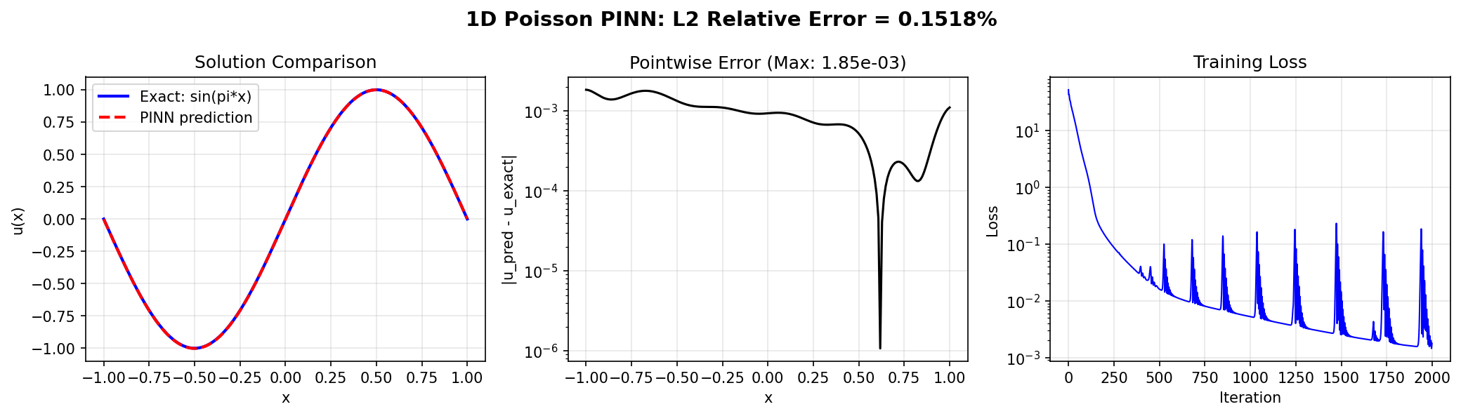
The plot shows:

Left: PINN prediction overlaid on exact solution (nearly identical)
Center: Pointwise absolute error on log scale (max ~1.9e-3)
Right: Training loss convergence over 2000 iterations

Results Summary¶

Metric	Value
L2 Absolute Error	0.001071
L2 Relative Error	0.1518%
Maximum Error	0.001853
Final Loss	1.77e-03
Parameters	5,251
Training Iterations	2,000
Runtime	~2-3 sec (GPU)

Next Steps¶

Experiments to Try¶

Increase iterations: Train for 5000+ iterations for even lower error
Vary architecture: Try hidden_dims=[100, 100] or [32, 32, 32, 32]
Adjust loss weights: Customize PINNConfig.loss_config for different BC enforcement
Custom residuals: Define your own residual function for any PDE

Example	Level	What You'll Learn
Poisson 2D	Intermediate	Same problem in 2D
Burgers Equation	Intermediate	Nonlinear PDE with shocks
Heat Equation	Intermediate	Time-dependent parabolic PDE
First Neural Operator	Beginner	Data-driven operator learning

API Reference¶

Interval — 1D geometry class
create_poisson_pinn — PINN factory function
PINNSolver — High-level PINN solver
PINNConfig — Solver configuration
poisson_residual — Poisson residual factory

Troubleshooting¶

Loss doesn't decrease¶

Symptom: Loss stays near initial value after many iterations.

Cause: Learning rate too low or network too small.

Solution: Increase learning rate or add more hidden units:

config = PINNConfig(
    learning_rate=1e-2,  # Higher learning rate
    num_iterations=2000,
)

# Or use larger network
pinn = create_poisson_pinn(
    spatial_dim=1,
    hidden_dims=[100, 100, 100],  # Larger
    rngs=nnx.Rngs(42),
)

Boundary conditions not satisfied¶

Symptom: Large error at x = -1 and x = 1.

Cause: BC loss weight too low relative to PDE loss.

Solution: Customize the loss_config in PINNConfig:

from opifex.core.physics.losses import PhysicsLossConfig

config = PINNConfig(
    loss_config=PhysicsLossConfig(
        physics_loss_weight=1.0,
        boundary_loss_weight=1000.0,  # Was 100.0
    ),
)

NaN in loss¶

Symptom: Loss becomes nan after a few iterations.

Cause: Learning rate too high or numerical instability.

Solution: Reduce learning rate:

config = PINNConfig(
    learning_rate=1e-4,  # Reduced from 1e-3
)

Your First PINN: Solving the Poisson Equation¶

Overview¶

What You'll Learn¶

Coming from DeepXDE?¶

Files¶

Quick Start¶

Run the Python Script¶

Run the Jupyter Notebook¶

Core Concepts¶

The PINN Paradigm¶

The Poisson Equation¶

Opifex PINN Architecture¶

Implementation¶

Step 1: Imports¶

Step 2: Define the Problem¶

Step 3: Define the Geometry¶

Step 4: Create the PINN Model¶

Step 5: Create PDE Residual¶

Step 6: Configure and Solve¶

Step 7: Evaluation¶

Visualization¶

Results Summary¶

Next Steps¶

Experiments to Try¶

Related Examples¶

API Reference¶

Troubleshooting¶

Loss doesn't decrease¶

Boundary conditions not satisfied¶

NaN in loss¶