Spectral Normalization: Lipschitz Control for Stable Deep Training
| Metadata | Value |
|---|---|
| Level | Intermediate |
| Runtime | ~1 min (GPU) / ~3 min (CPU) |
| Prerequisites | JAX, Flax NNX, basic optimisation |
| Format | Python + Jupyter |
| Memory | ~0.5 GB |
Overview
Spectral normalization (Miyato et al. 2018, Spectral Normalization for Generative Adversarial Networks, arXiv:1802.05957) divides each weight matrix by its largest singular value, making every layer 1-Lipschitz. The product of per-layer spectral norms upper-bounds the whole network's Lipschitz constant — and an unbounded Lipschitz constant is exactly what makes deep networks blow up at aggressive learning rates.
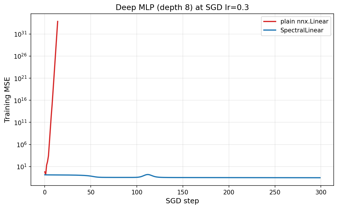
This example demonstrates that value with a controlled comparison: a deep MLP trained at an
aggressive learning rate, built once with plain nnx.Linear layers and once with
SpectralLinear. We track the training loss and the network Lipschitz
bound (the product of per-layer spectral norms). The plain network's Lipschitz bound starts above
1000 and its training diverges to NaN; the spectral-normalized network keeps every layer at
spectral norm 1 and trains stably to a low error.
What You'll Learn
- Use
SpectralLinearas a drop-in 1-Lipschitz replacement fornnx.Linear - Measure a network's Lipschitz bound as the product of per-layer spectral norms
- See how Lipschitz control stabilises deep training at aggressive learning rates
Files
- Python Script:
examples/layers/spectral_normalization_example.py - Jupyter Notebook:
examples/layers/spectral_normalization_example.ipynb
Quick Start
Coming from PyTorch?
| PyTorch | Opifex |
|---|---|
torch.nn.utils.parametrizations.spectral_norm(nn.Linear(...)) |
SpectralLinear(in_features=, out_features=, power_iterations=, rngs=) |
spectral_norm(nn.Conv2d(...)) |
SpectralNormalizedConv(in_channels=, out_channels=, kernel_size=, rngs=) |
The Comparison
Both networks are the same deep MLP (width 64, depth 8, tanh activations); only the layer type
differs. SpectralLinear normalises each kernel by its spectral norm (via power iteration) before
the matmul, so the layer is 1-Lipschitz by construction. Both are trained with full-batch SGD at
an aggressive lr=0.3 on a gently-sloped regression target (so the 1-Lipschitz network has ample
capacity — the comparison isolates stability, not capacity).
class DeepMLP(nnx.Module):
    def __init__(self, width, depth, *, spectral, rngs):
        dims = [1, *([width] * depth), 1]
        layers = [
            (SpectralLinear(a, b, power_iterations=2, rngs=rngs) if spectral
             else nnx.Linear(a, b, rngs=rngs))
            for a, b in pairwise(dims)
        ]
        self.layers = nnx.List(layers)
Results
Terminal Output:
Lipschitz bound at init:  plain=1.01e+03  spectral=1.00e+00

========================================================================
RESULTS
========================================================================
Model                          final MSE       max MSE   Lipschitz bound
------------------------------------------------------------------------
plain nnx.Linear                     nan           nan               nan
SpectralLinear                2.9396e-02    1.5593e-01          1.00e+00
------------------------------------------------------------------------
Plain network destabilised: True; spectral final MSE 2.94e-02 (Lipschitz bound stays ~1 per layer).
| Model | Final MSE | Lipschitz bound | Outcome |
|---|---|---|---|
plain nnx.Linear |
NaN | unbounded (≈10³ at init) | diverges |
SpectralLinear |
0.029 | 1.0 per layer | stable |
The plain deep network has a Lipschitz bound over 1000 at initialisation; at lr=0.3 it blows up
to NaN within the first few steps. Spectral normalization caps every layer at spectral norm 1, so
the network is globally Lipschitz-bounded and trains stably to a low MSE — at no extra parameters,
just a power-iteration estimate per layer.
Stability vs capacity
1-Lipschitz layers trade some expressivity for stability — a strict Lipschitz bound limits how
steep a function the network can represent. The target here is deliberately gentle so capacity
is not the bottleneck; for steeper targets, relax the constraint (fewer normalized layers) or
use AdaptiveSpectralNorm, which learns a per-layer bound.
Next Steps
Experiments to Try
- Lower the learning rate until the plain network also trains — find the stability threshold.
- Swap in
SpectralNormalizedConvand repeat with a small CNN. - Try
AdaptiveSpectralNorm(learnable bound) to recover capacity while keeping stability.
Related Examples
- Grid Embeddings — another neural-operator building block, measured.
- FNO on Darcy Flow — where spectral layers are used in anger.