Variational Monte Carlo: H, He and H2 ground states¶

Metadata	Value
Level	Advanced
Runtime	~2 min (GPU, jit + lax.scan sampler)
Prerequisites	JAX, Flax NNX, variational Monte Carlo, neural wavefunctions
Format	Python + Jupyter
Memory	~2 GB RAM

Overview¶

This example recovers the ground-state energies of the hydrogen atom, the helium atom, and the hydrogen molecule from first principles with variational Monte Carlo (VMC), using a FermiNet neural-network wavefunction (Pfau et al. 2020, arXiv:1909.02487). VMC minimises the variational energy

E[theta] = < E_loc >_{|psi_theta|^2},   E_loc(r) = (H psi_theta)(r) / psi_theta(r)

of a trial wavefunction psi_theta by stochastic gradient descent on its parameters, with the expectation taken over walkers sampled from the Born density |psi_theta|^2. By the variational principle the energy is an upper bound on the true ground state, so lower is always better — there is no label set to overfit, and matching the exact reference is a faithful recovery of known physics.

These three systems have essentially exact references (H -0.5, He -2.9037 (Pekeris 1958), H2 at R=1.4 bohr -1.1745 Hartree), so the goal here is faithful recovery to chemical accuracy (better than 1 mHa), not beating a benchmark. The identical ansatz, sampler and optimiser scale unchanged to larger molecules where no exact answer exists.

The example is deliberately thin — it composes opifex's committed VMC stack and changes no library internals:

FermiNet is the generalized-Slater equivariant ansatz, evaluated in the log domain one walker at a time and vmap-ed over the batch.
MetropolisHastingsSampler draws walkers from |psi|^2 with the FermiNet harmonic-mean proposal, fusing all MCMC sweeps into one jax.lax.scan.
VMCDriver runs the energy-minimisation loop: each jitted step samples walkers, evaluates the per-walker local energy (forward-Laplacian kinetic term), and applies a SPRING natural-gradient update.
VMCConfig selects the SPRING optimiser, the batch size and the iteration budget.

What You'll Learn¶

Build a FermiNet wavefunction for an atom or molecule
Sample the Born density |psi|^2 with the harmonic-mean Metropolis sampler
Minimise the variational energy with the SPRING natural-gradient optimiser
Recover H, He and H2 ground-state energies to chemical accuracy
Read the energy-convergence curve and the sampled walker density

Background: variational Monte Carlo¶

VMC turns the Schrödinger eigenvalue problem into an optimisation. For any trial wavefunction the local energy E_loc(r) = (H psi)(r) / psi(r) is a function of a single electron configuration r, and its average over the Born density |psi|^2 equals the variational energy E[theta]. The variational principle guarantees E[theta] >= E_0, the exact ground state, with equality only at the true ground-state wavefunction. So minimising E[theta] drives psi_theta toward the ground state, and the recovered energy is always an upper bound.

opifex evaluates the local energy with a native forward-Laplacian kinetic term — the Hessian diagonal of log|psi| obtained from stacked JVPs in O(1) forward passes (the LapNet speed-up) rather than O(n) reverse-then-forward passes. The gradient signal is the FermiNet score-function estimator grad E = 2 < (E_loc - <E_loc>) grad log|psi| >, preconditioned by the SPRING natural gradient. See Variational Monte Carlo for the backbone → local-energy → optimiser design.

Configuration¶

Each system is described by its nuclear geometry (in bohr), charges, spin partition (n_up, n_down), exact reference, and a per-system optimisation budget. The ansatz, sampler and optimiser hyper-parameters are shared across all three systems and follow the FermiNet small-atom recipe: a two-layer equivariant backbone (one-electron widths (32, 32), two-electron widths (16, 16)) with four generalized-Slater determinants, the SPRING optimiser, and a 1024-walker harmonic-mean Metropolis sampler with 10 sweeps per step.

from dataclasses import dataclass
import jax
import jax.numpy as jnp

# float64 + matmul precision "high": VMC energies are validated to ~1 mHa, well
# below the TF32 fallback error on GPU.
jax.config.update("jax_enable_x64", True)
jax.config.update("jax_default_matmul_precision", "high")


@dataclass(frozen=True, slots=True, kw_only=True)
class System:
    name: str
    atoms: jax.Array
    charges: jax.Array
    nspins: tuple[int, int]
    exact_energy: float
    iterations: int
    learning_rate: float
    seed: int


SYSTEMS = (
    System(name="H", atoms=jnp.array([[0.0, 0.0, 0.0]]), charges=jnp.array([1.0]),
           nspins=(1, 0), exact_energy=-0.5, iterations=400, learning_rate=0.05, seed=0),
    System(name="He", atoms=jnp.array([[0.0, 0.0, 0.0]]), charges=jnp.array([2.0]),
           nspins=(1, 1), exact_energy=-2.9037, iterations=800, learning_rate=0.04, seed=2),
    System(name="H2", atoms=jnp.array([[0.0, 0.0, 0.0], [0.0, 0.0, 1.4]]),
           charges=jnp.array([1.0, 1.0]), nspins=(1, 1), exact_energy=-1.1745,
           iterations=600, learning_rate=0.05, seed=1),
)

Building one VMC run¶

A VMC run for any system is the same three-object composition: a FermiNet ansatz, a MetropolisHastingsSampler, and a VMCDriver carrying the VMCConfig. The ansatz exposes a single-walker positions -> (sign, log|psi|) call (log domain for stability); the driver vmaps it over the walker batch for sampling and the local energy, and grads it for the score-function gradient and the per-sample Jacobian the SPRING solve needs. Spin (n_up, n_down) is a static attribute, so the whole step is one jit-compiled GPU kernel.

from flax import nnx
from opifex.neural.quantum.vmc import (
    FermiNet, MetropolisHastingsSampler, VMCConfig, VMCDriver,
)


def build_driver(system):
    ansatz = FermiNet(
        nspins=system.nspins, atoms=system.atoms, charges=system.charges,
        hidden_one=(32, 32), hidden_two=(16, 16),
        determinants=4, full_det=True, rngs=nnx.Rngs(system.seed),
    )
    sampler = MetropolisHastingsSampler(atoms=system.atoms, steps=10, step_size=0.4)
    config = VMCConfig(
        batch_size=1024, iterations=system.iterations, optimizer="spring",
        learning_rate=system.learning_rate, equilibration_steps=200,
    )
    return VMCDriver(ansatz=ansatz, sampler=sampler, config=config)

Training¶

VMCDriver.run equilibrates the walkers under the freshly initialised wavefunction, then runs iterations jitted optimisation steps. Each step

advances the walkers by 10 Metropolis-Hastings sweeps (one fused lax.scan) so they track the current |psi_theta|^2;
evaluates the per-walker local energy with the native forward-Laplacian kinetic term, with outlier-robust median-absolute-deviation clipping; then
forms the FermiNet score-function energy gradient, preconditions it with the SPRING natural-gradient solve (Fisher inverse in sample space + Nesterov momentum), and updates the parameters.

The reported energy is the mean local energy over the final batch with its Monte Carlo standard error sigma / sqrt(N).

import jax

results = {}
for system in SYSTEMS:
    driver = build_driver(system)
    results[system.name] = driver.run(jax.random.PRNGKey(system.seed))

The SPRING natural gradient is what makes this fast: it preconditions the energy gradient by the inverse Fisher matrix, solved in the cheap sample space (an N x N Gram system, not a parameter-space one), and adds Nesterov momentum — so the energy reaches chemical accuracy in a few hundred iterations rather than the thousands a plain first-order optimiser would need.

Results¶

Recovered energies on a single GPU run of this example (float64, matmul precision high), against the essentially-exact references. Chemical accuracy is the conventional 1 kcal/mol ~ 1.594 mHa threshold; the variational principle bounds every recovered energy from above, so the errors are essentially all positive (above the true ground state) up to Monte Carlo noise.

======================================================================
VMC ground-state energies vs exact references
======================================================================
System |           E_VMC (Ha) |  Exact (Ha) |      Error |   Status
-------------------------------------------------------------------
     H | -0.49956 +/- 0.00002 |     -0.5000 |   +0.44 mHa | chem-acc
    He | -2.90369 +/- 0.00008 |     -2.9037 |   +0.01 mHa | chem-acc
    H2 | -1.17448 +/- 0.00012 |     -1.1745 |   +0.02 mHa | chem-acc
-------------------------------------------------------------------
Chemical accuracy threshold: |error| < 1.594 mHa (1 kcal/mol)

System	E_VMC (Ha)	Exact (Ha)	Error	Reference
H	-0.49956 ± 0.00002	-0.5000	+0.44 mHa	exact `-1/2`
He	-2.90369 ± 0.00008	-2.9037	+0.01 mHa	Pekeris 1958 (essentially exact)
H2	-1.17448 ± 0.00012	-1.1745	+0.02 mHa	exact Born-Oppenheimer @ R=1.4 bohr

All three land inside chemical accuracy — He and H2 to a few hundredths of a milli-Hartree, H to under half a milli-Hartree. The whole run (three systems, 400/800/600 iterations) takes about 82 seconds of compute on a single GPU plus jit compilation. These are recoveries of known physics, not a benchmark score: because the variational principle bounds every energy from above, recovering the exact references to under 1 mHa is direct evidence the ansatz, sampler and optimiser are correct and accurate — and the same stack scales, unchanged, to molecules where no exact answer exists.

Energy convergence¶

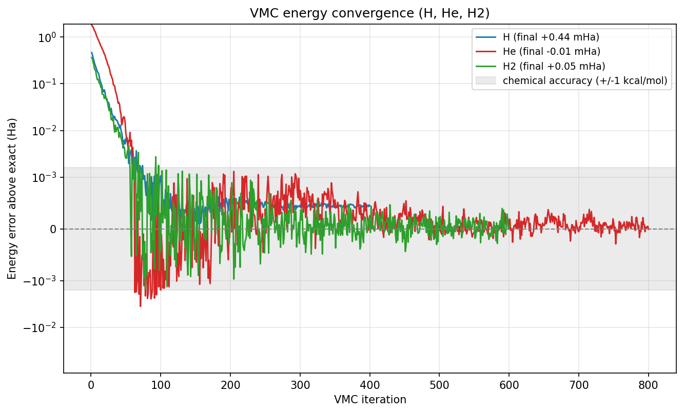
Energy error above the exact reference per VMC iteration for H, He and H2 on a symmetric-log axis, with the chemical-accuracy band shaded; all three curves decay from ~1 Hartree into the band within a few hundred iterations

The error above the exact reference is plotted on a symmetric-log axis so both the early macroscopic descent and the final sub-milli-Hartree convergence are visible. All three systems fall from ~1 Hartree into the shaded chemical-accuracy band (±1 kcal/mol) within a few hundred SPRING iterations and then fluctuate around zero at the Monte Carlo noise floor.

Hydrogen walker density¶

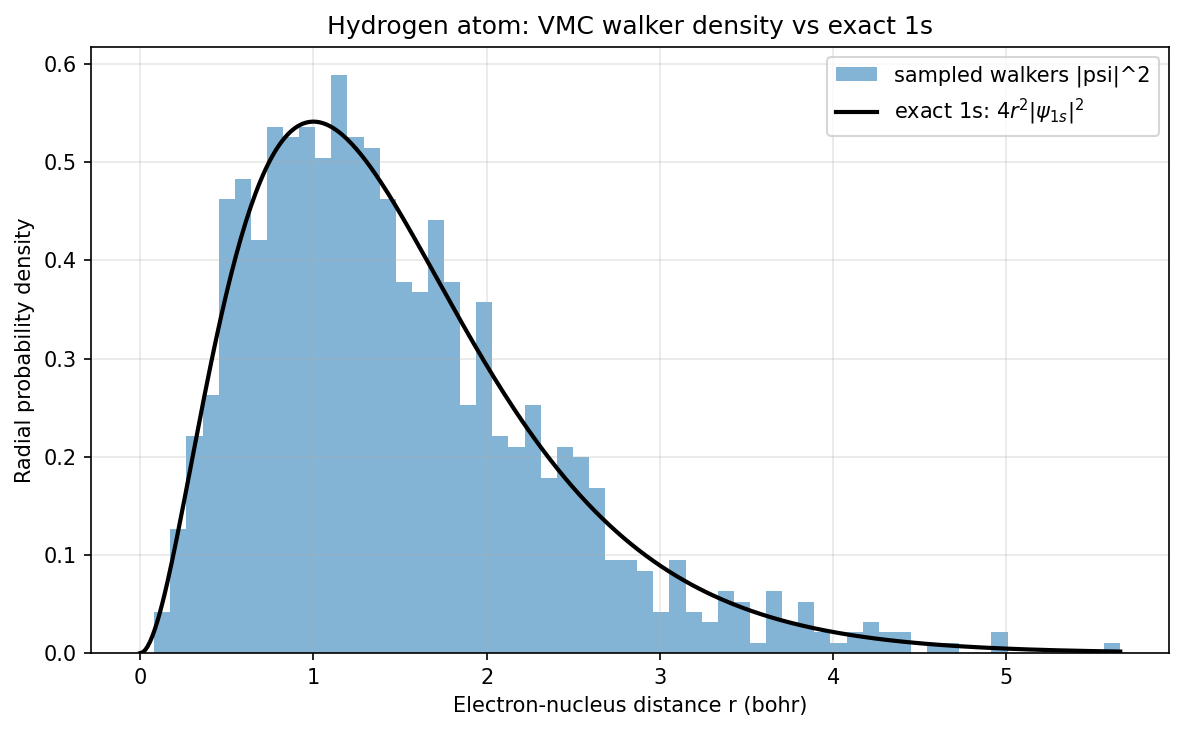
Radial probability density of the converged hydrogen walkers (histogram) overlaid with the exact 1s radial distribution 4 r^2 |psi_1s|^2, peaking at the Bohr radius r = 1; the histogram tracks the exact curve closely

A direct check that the Metropolis sampler draws from the correct Born density: the converged hydrogen walkers' radial distribution matches the exact hydrogen 1s radial density 4 r^2 |psi_1s|^2 (with psi_1s = exp(-r) / sqrt(pi)), peaking at the Bohr radius r = 1.

Running the example¶

uv run python examples/quantum-chemistry/vmc_atoms.py

The run is self-contained — no dataset download. It enables float64 and pins the matmul precision to high so the GPU float32 (TF32) fallback does not pollute the milli-Hartree energies.

Key takeaways¶

A VMC ground-state calculation is a thin composition of the opifex VMC stack: FermiNet ansatz → MetropolisHastingsSampler → VMCDriver with the SPRING optimiser → energy table and plots.
The variational principle makes this honest — every recovered energy is an upper bound on the exact ground state, so matching the references to <1 mHa is a faithful recovery of known physics, not a fit to labels.
The forward-Laplacian local energy gives the kinetic term in O(1) forward passes, and the whole optimisation step (sampler lax.scan + local energy + SPRING update) is one jit-compiled GPU kernel.
SPRING natural gradient converges fast — preconditioning by the inverse Fisher matrix in sample space plus Nesterov momentum reaches chemical accuracy in a few hundred iterations rather than thousands.
The same stack scales unchanged to larger molecules; for bigger systems, swap in a PsiFormer attention backbone, a MALA sampler, or larger walker counts.