Heat Equation PINN

Metadata	Value
Level	Intermediate
Runtime	~1 min (GPU) / ~5 min (CPU)
Prerequisites	JAX, Flax NNX, basic calculus
Format	Python + Jupyter
Memory	~500 MB RAM

Overview

Physics-Informed Neural Networks (PINNs) solve PDEs by embedding the governing equations directly into the neural network loss function. Instead of learning from labeled input-output pairs, PINNs minimize the PDE residual at collocation points, requiring no simulation data.

This example demonstrates solving the heat equation \(\frac{\partial u}{\partial t} = \alpha \nabla^2 u\) on a 2D rectangular domain using Opifex's PINN infrastructure. It covers problem definition with geometry primitives, model creation, collocation-based training, and loss evaluation.

What You'll Learn

1. Define a PDE problem with create_pde_problem and geometry primitives
2. Create a PINN model with create_heat_equation_pinn
3. Train using Opifex's Trainer with collocation points
4. Evaluate training results and loss convergence

Coming from DeepXDE?

DeepXDE	Opifex (JAX)
dde.geometry.Rectangle([0,0], [1,1])	Rectangle(center=jnp.array([0.5, 0.5]), width=1.0, height=1.0)
dde.data.PDE(geom, pde, bc, ...)	create_pde_problem(geometry=, equation=, boundary_conditions=)
dde.Model(data, net)	create_heat_equation_pinn(spatial_dim=2, hidden_dims=[50,50,50], rngs=)
model.compile("adam", lr=1e-3)	TrainingConfig(num_epochs=100, learning_rate=1e-3)
model.train(epochs=10000)	trainer.fit(train_data=(x, y))
dde.grad.jacobian(y, x, i=0, j=0)	jax.grad(u_fn, argnums=0)(x, t)

Key difference: Opifex uses JAX's automatic differentiation directly (jax.grad, jax.hessian), which is more composable than DeepXDE's gradient API. PDE residuals are computed as pure functions, enabling JIT compilation of the entire training loop.

Files

• Python Script: examples/pinns/heat_equation.py
• Jupyter Notebook: examples/pinns/heat_equation.ipynb

Quick Start

Run the Python Script

source activate.sh && python examples/pinns/heat_equation.py

Run the Jupyter Notebook

jupyter lab examples/pinns/heat_equation.ipynb

Core Concepts

How PINNs Work

PINNs replace traditional PDE solvers by training a neural network to satisfy the governing equation. The loss function has three components:

graph TB
    A["Collocation Points<br/>(random in domain)"] --> B["Neural Network<br/>u_theta(x, t)"]
    B --> C["PDE Residual Loss<br/>|du/dt - alpha * laplacian(u)|^2"]
    B --> D["Boundary Loss<br/>|u(x_boundary) - g(x)|^2"]
    B --> E["Initial Condition Loss<br/>|u(x, 0) - u_0(x)|^2"]
    C --> F["Total Loss"]
    D --> F
    E --> F

    style A fill:#e3f2fd
    style F fill:#c8e6c9

Heat Equation

The heat equation models diffusion processes:

\[\frac{\partial u}{\partial t} = \alpha \nabla^2 u\]

where \(\alpha\) is the thermal diffusivity and \(u(x,t)\) is the temperature field.

Component	This Example
Domain	\([0,1] \times [0,1]\) rectangle
Boundary	Dirichlet: \(u = 0\) on all boundaries
Diffusivity	\(\alpha = 0.01\)
Architecture	MultiScalePINN with 3 scale networks of 50 units

Implementation

Step 1: Define the PDE Problem

Use Opifex geometry primitives and problem definition:

from opifex.geometry import Rectangle
from opifex.core.problems import create_pde_problem

geometry = Rectangle(center=jax.numpy.array([0.5, 0.5]), width=1.0, height=1.0)

problem = create_pde_problem(
    geometry=geometry,
    equation=lambda x, u, u_x: 0.0,
    boundary_conditions=[{"type": "dirichlet", "boundary": "all", "value": 0.0}],
    parameters={"diffusivity": 0.01},
)

Step 2: Create the PINN Model

from opifex.neural.pinns import create_heat_equation_pinn

rngs = nnx.Rngs(42)
pinn = create_heat_equation_pinn(
    spatial_dim=2,
    hidden_dims=[50, 50, 50],
    rngs=rngs,
)

Step 3: Configure Training

from opifex.core.training.config import TrainingConfig
from opifex.core.training.trainer import Trainer

config = TrainingConfig(
    num_epochs=100,
    learning_rate=1e-3,
    batch_size=256,
)

trainer = Trainer(model=pinn, config=config)

Step 4: Generate Collocation Points and Train

key = jax.random.PRNGKey(42)
x = jax.random.uniform(key, (1000, 3))  # (x, y, t)
y = jax.numpy.zeros((1000, 1))          # Target: residual = 0

trainer.fit(train_data=(x, y))

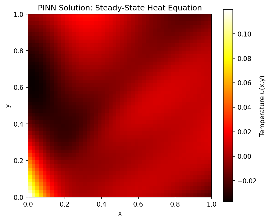
Visualization

The trained PINN's temperature field on the evaluation grid:

Results Summary

Metric	Value
Domain	\([0,1] \times [0,1]\)
PINN Architecture	[50, 50, 50]
Training Epochs	100
Learning Rate	1e-3
Batch Size	256
Diffusivity	0.01

Key Takeaways

• PINNs solve PDEs without simulation data by minimizing physics residuals
• Opifex provides factory functions for common PDE types (create_heat_equation_pinn)
• JAX's grad and hessian enable efficient PDE residual computation
• The Trainer handles optimization, while collocation points serve as "data"
• For better accuracy, increase epochs to 1000+ and use more collocation points

Next Steps

Experiments to Try

1. More epochs: Train for 1000-10000 epochs to observe convergence
2. Larger network: Try hidden_dims=[100, 100, 100, 100] for higher accuracy
3. Time-dependent: Add time dimension for transient heat equation
4. Adaptive sampling: Concentrate collocation points near boundaries

Related Examples

Example	Level	What You'll Learn
Domain Decomposition PINNs	Advanced	Scale PINNs to large domains
FNO Darcy Full	Intermediate	Data-driven alternative to PINNs
Enhanced Calibration	Advanced	Uncertainty quantification for predictions

API Reference

• create_pde_problem - PDE problem definition factory
• create_heat_equation_pinn - Heat equation PINN factory
• Rectangle - 2D rectangular geometry
• Trainer - Training orchestration
• TrainingConfig - Training hyperparameters

Troubleshooting

Loss not decreasing

Symptom: Training loss stays flat after many epochs.

Cause: Learning rate too low, or insufficient collocation points.

Solution: Increase learning rate to 1e-2 for initial training, then reduce. Use at least 1000 collocation points for a 2D domain:

config = TrainingConfig(num_epochs=1000, learning_rate=1e-2, batch_size=512)

PINN predicts zero everywhere

Symptom: All predictions are approximately zero.

Cause: Boundary loss dominates, pushing the solution to the trivial solution.

Solution: Balance loss components. Use adaptive loss weighting:

# Weight physics loss higher than boundary loss
total_loss = 10.0 * physics_loss + 1.0 * boundary_loss

Slow training on CPU

Symptom: Each epoch takes seconds instead of milliseconds.

Cause: No JIT compilation, or small batch sizes preventing vectorization.

Solution: Ensure JIT compilation is active (it is by default with Opifex's Trainer). Use batch sizes of 256+ for efficient vectorization.