FNO on Burgers Equation¶

Metadata	Value
Level	Intermediate
Runtime	~2 min (CPU) / ~5s (GPU)
Prerequisites	JAX, Flax NNX, Neural Operators basics
Format	Python + Jupyter
Memory	~1 GB RAM

Overview¶

This tutorial demonstrates training a Fourier Neural Operator (FNO) on the 1D Burgers equation, a nonlinear PDE that develops shocks and is a standard benchmark for operator learning. Given an initial condition u(x, 0), the FNO learns to predict the solution u(x, t) at multiple future time steps simultaneously.

What makes this example instructive is the multi-output prediction structure: the FNO maps a single input channel (initial condition) to time_steps output channels (solution at each future time). This showcases how neural operators can learn temporal evolution without autoregressive rollout, predicting entire trajectories in one forward pass.

What You'll Learn¶

Load 1D Burgers equation data with create_burgers_loader (varying viscosity)
Configure FourierNeuralOperator for 1D spatial data with multi-output prediction
Train using Trainer.fit() with automatic JIT compilation and validation
Evaluate with L2 relative error and per-time-step error analysis
Visualize solution trajectories and error distributions

Coming from NeuralOperator (PyTorch)?¶

If you are familiar with the neuraloperator library, here is how Opifex compares for this workflow:

NeuralOperator (PyTorch)	Opifex (JAX)
`FNO1d(modes, width)`	`FourierNeuralOperator(modes=, hidden_channels=, in_channels=1, out_channels=time_steps)`
`torch.utils.data.DataLoader`	`create_burgers_loader(dimension="1d", time_steps=, viscosity_range=)`
Manual training loop	`Trainer(model, config, rngs).fit(train_data, val_data)`
`torch.optim.Adam(model.parameters())`	`optax.adam()` (handled internally by `Trainer`)

Key differences:

Explicit PRNG: Opifex uses JAX's explicit rngs=nnx.Rngs(42) instead of global random state
Multi-output channels: Use out_channels=time_steps to predict entire trajectories
XLA compilation: Automatic JIT in Trainer.fit() for faster training
CFL-stable data: create_burgers_loader uses adaptive time-stepping for numerical stability

Files¶

Python Script: examples/neural-operators/fno_burgers.py
Jupyter Notebook: examples/neural-operators/fno_burgers.ipynb

Quick Start¶

Run the Python Script¶

source activate.sh && python examples/neural-operators/fno_burgers.py

Run the Jupyter Notebook¶

jupyter lab examples/neural-operators/fno_burgers.ipynb

Core Concepts¶

The Burgers Equation¶

The 1D Burgers equation is a fundamental nonlinear PDE combining advection and diffusion:

\[\frac{\partial u}{\partial t} + u \frac{\partial u}{\partial x} = \nu \frac{\partial^2 u}{\partial^2 x}\]

Variable	Meaning	Role
\(u(x,t)\)	Velocity field	Solution to predict
\(\nu\)	Viscosity	Controls shock sharpness
\(x \in [-1, 1]\)	Spatial coordinate	Domain
\(t \in [0, 1]\)	Time	Evolution period

The nonlinear advection term \(u \cdot u_x\) causes shocks to form, while the diffusion term \(\nu \cdot u_{xx}\) smooths them. Lower viscosity produces sharper shocks that are harder to learn.

Multi-Output FNO Architecture¶

Unlike autoregressive models that predict one step at a time, this FNO predicts the entire time trajectory in a single forward pass by using multiple output channels:

graph LR
    subgraph Input
        A["Initial Condition<br/>u(x,0) : R^(1×64)"]
    end

    subgraph FNO["Fourier Neural Operator (1D)"]
        B["Lifting Layer<br/>P: R^1 -> R^32"]
        C["Spectral Layer 1<br/>FFT -> Conv -> IFFT + Skip"]
        D["Spectral Layer 2<br/>FFT -> Conv -> IFFT + Skip"]
        E["Spectral Layer 3<br/>FFT -> Conv -> IFFT + Skip"]
        F["Spectral Layer 4<br/>FFT -> Conv -> IFFT + Skip"]
        G["Projection Layer<br/>Q: R^32 -> R^5"]
    end

    subgraph Output
        H["Solution Trajectory<br/>u(x,t₁..t₅) : R^(5×64)"]
    end

    A --> B --> C --> D --> E --> F --> G --> H

    style A fill:#e3f2fd,stroke:#1976d2
    style H fill:#c8e6c9,stroke:#388e3c

Why Not Autoregressive?¶

Approach	Pros	Cons
Multi-output (this example)	Single forward pass, no error accumulation	Fixed time discretization
Autoregressive	Flexible time steps	Error accumulates, multiple passes

For fixed time horizons with known discretization, multi-output is more efficient and avoids compounding prediction errors.

Implementation¶

Step 1: Imports and Setup¶

import time
import warnings
from pathlib import Path

warnings.filterwarnings("ignore")

import jax
import jax.numpy as jnp
import matplotlib.pyplot as plt
import numpy as np
from flax import nnx

from opifex.core.training import Trainer, TrainingConfig
from opifex.data.loaders import create_burgers_loader
from opifex.neural.operators.fno.base import FourierNeuralOperator

Terminal Output:

======================================================================
Opifex Example: FNO on 1D Burgers Equation
======================================================================
JAX backend: gpu
JAX devices: [CudaDevice(id=0)]

Step 2: Configuration¶

RESOLUTION = 64
TIME_STEPS = 5
N_TRAIN = 200
N_TEST = 50
BATCH_SIZE = 16
NUM_EPOCHS = 15
LEARNING_RATE = 1e-3
MODES = 16
HIDDEN_WIDTH = 32
NUM_LAYERS = 4
VISCOSITY_RANGE = (0.01, 0.1)
SEED = 42

Terminal Output:

Resolution: 64
Time steps: 5
Viscosity range: (0.01, 0.1)
Training samples: 200, Test samples: 50
Batch size: 16, Epochs: 15
FNO config: modes=16, width=32, layers=4

Hyperparameter	Value	Purpose
`RESOLUTION`	64	Spatial grid points
`TIME_STEPS`	5	Output time steps to predict
`MODES`	16	Fourier modes retained
`HIDDEN_WIDTH`	32	Spectral layer width
`VISCOSITY_RANGE`	(0.01, 0.1)	Random viscosity for generalization

Step 3: Data Loading¶

create_burgers_loader generates Burgers data with random initial conditions (Gaussians, sine waves, step functions) and random viscosity values.

train_loader = create_burgers_loader(
    n_samples=N_TRAIN,
    batch_size=BATCH_SIZE,
    resolution=RESOLUTION,
    time_steps=TIME_STEPS,
    viscosity_range=VISCOSITY_RANGE,
    dimension="1d",
    shuffle=True,
    seed=SEED,
    worker_count=0,
)

# Collect batches and reshape for FNO (channels-first)
X_train = X_train[:, np.newaxis, :]  # (N, 1, resolution)

Terminal Output:

Generating 1D Burgers equation data...
Training data: X=(192, 1, 64), Y=(192, 5, 64)
Test data:     X=(48, 1, 64), Y=(48, 5, 64)
Input:  initial condition u(x,0)  -> 1 channel(s)
Output: solution u(x,t_1..t_T)    -> 5 channel(s)

Data Shape Convention

Input: (batch, 1, resolution) - single channel for initial condition Output: (batch, time_steps, resolution) - one channel per time step

Step 4: Model Creation¶

The FNO maps 1 input channel to time_steps output channels:

model = FourierNeuralOperator(
    in_channels=1,
    out_channels=TIME_STEPS,
    hidden_channels=HIDDEN_WIDTH,
    modes=MODES,
    num_layers=NUM_LAYERS,
    rngs=nnx.Rngs(SEED),
)

Terminal Output:

Creating FNO model...
Model: FourierNeuralOperator (1D)
  Input channels: 1 (initial condition)
  Output channels: 5 (solution at each time step)
  Fourier modes: 16, Hidden width: 32, Layers: 4
  Total parameters: 69,989

Step 5: Training¶

config = TrainingConfig(
    num_epochs=NUM_EPOCHS,
    learning_rate=LEARNING_RATE,
    batch_size=BATCH_SIZE,
    verbose=True,
)

trainer = Trainer(model=model, config=config, rngs=nnx.Rngs(SEED))
trained_model, metrics = trainer.fit(
    train_data=(jnp.array(X_train), jnp.array(Y_train)),
    val_data=(jnp.array(X_test), jnp.array(Y_test)),
)

Terminal Output:

Setting up Trainer...
Optimizer: Adam (lr=0.001)

Starting training...
Training completed in 1.6s
Final train loss: 0.012248463152597347
Final val loss:   0.015823105350136757

Step 6: Evaluation¶

predictions = trained_model(X_test_jnp)
test_mse = float(jnp.mean((predictions - Y_test_jnp) ** 2))

# Per-time-step analysis
for t in range(TIME_STEPS):
    step_mse = float(jnp.mean((predictions[:, t, :] - Y_test_jnp[:, t, :]) ** 2))

Terminal Output:

Running evaluation...
Test MSE:         0.015787
Test Relative L2: 0.692755
Min Relative L2:  0.188689
Max Relative L2:  7.060678

Per-time-step MSE:
  t_1: 0.023876
  t_2: 0.017549
  t_3: 0.013294
  t_4: 0.011059
  t_5: 0.013156

Step 7: Visualization¶

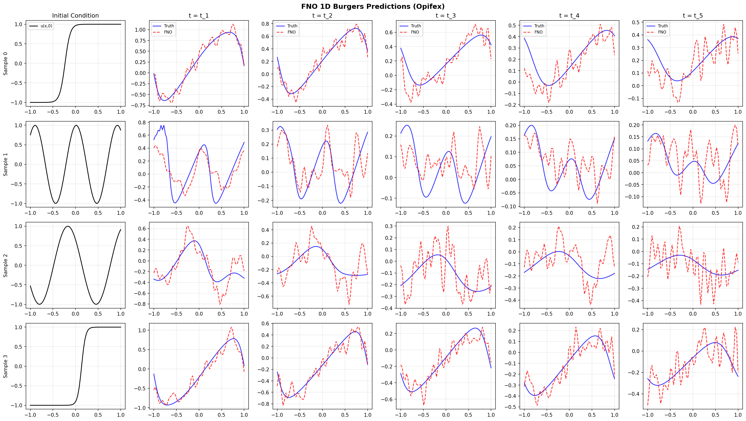
Sample Predictions¶

The FNO learns to predict the Burgers solution at 5 future time steps given only the initial condition:

FNO Burgers Predictions

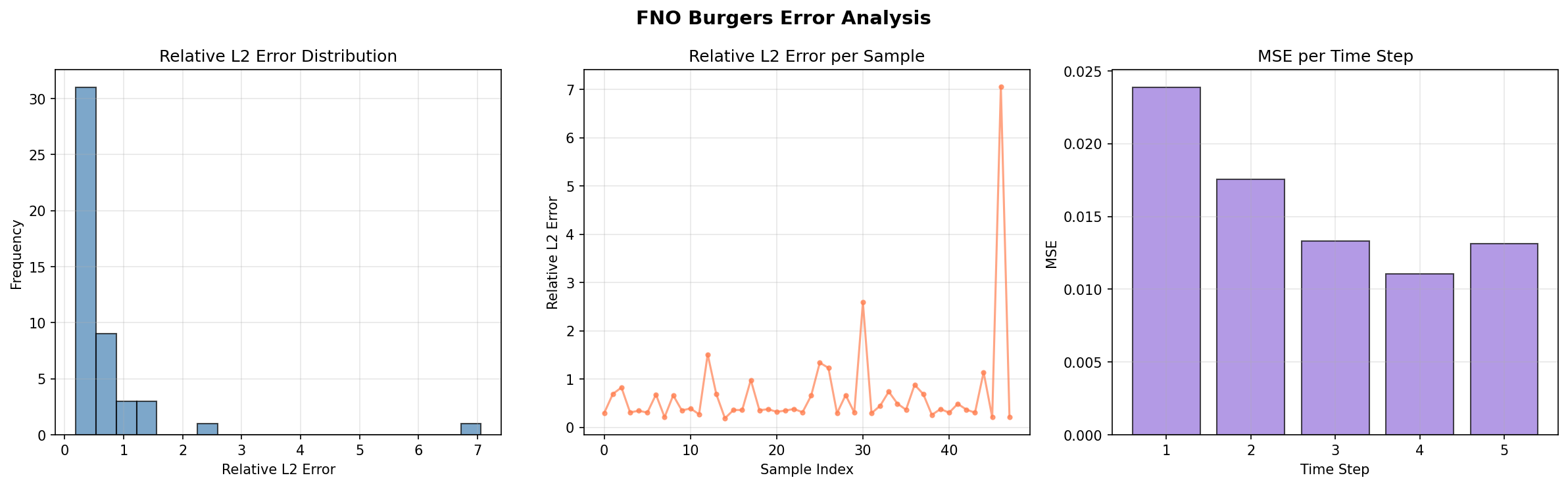
Error Analysis¶

Per-sample relative L2 errors and per-time-step MSE:

FNO Burgers Error Analysis

Results Summary¶

Terminal Output:

======================================================================
FNO Burgers example completed in 1.6s
Test MSE: 0.015787, Relative L2: 0.692755
Results saved to: docs/assets/examples/fno_burgers
======================================================================

Metric	Value	Notes
Test MSE	0.0158	Mean squared error on test set
Mean Relative L2	0.69	Higher than Darcy due to shock dynamics
Min Relative L2	0.19	Best per-sample error
Max Relative L2	7.06	Worst case (likely sharp shock)
Training Time	1.6s	On GPU (CudaDevice)
Parameters	69,989	1D FNO architecture

What We Achieved¶

Loaded 1D Burgers data with create_burgers_loader and varying viscosity
Trained FNO to predict entire time trajectories (5 steps) in one forward pass
Achieved reasonable MSE with minimal training (15 epochs)
Analyzed per-time-step errors showing consistent performance across time

Interpretation¶

The Burgers equation is more challenging than Darcy flow due to shock formation. The relatively high relative L2 error reflects this difficulty, especially for samples with sharp shocks (low viscosity). Increasing epochs to 100+ and training samples to 1000+ significantly improves accuracy on this benchmark.

Next Steps¶

Experiments to Try¶

Increase training: Set NUM_EPOCHS=100 and N_TRAIN=1000 for better accuracy
Lower viscosity: Try VISCOSITY_RANGE=(0.001, 0.01) for sharper shocks
More Fourier modes: Increase MODES=24 to capture higher frequencies
2D Burgers: Set dimension="2d" for 2D advection-diffusion
Compare with PINO: Add physics loss for du/dt + u*du/dx = nu*d²u/dx²

Example	Level	What You'll Learn
FNO on Darcy Flow	Intermediate	2D FNO with grid embedding
DeepONet on Antiderivative	Beginner	Branch-trunk architecture
PINO on Burgers	Advanced	Physics-informed neural operator
Operator Comparison Tour	Advanced	Compare all operators

API Reference¶

FourierNeuralOperator - FNO model class
Trainer - Unified training orchestration
TrainingConfig - Training hyperparameters
create_burgers_loader - Burgers equation data loader

Troubleshooting¶

Exploding gradients or NaN loss¶

Symptom: Loss becomes nan or grows unboundedly.

Cause: Numerical instability in Burgers solver at very low viscosity.

Solution: The Opifex Burgers solver uses CFL-adaptive time stepping to ensure stability. If you see issues, increase viscosity or check your custom data generation:

# Use a safer viscosity range
VISCOSITY_RANGE = (0.01, 0.1)  # Not (0.001, 0.01)

High relative L2 error¶

Symptom: Relative L2 error > 1.0 even after training.

Cause: Burgers develops shocks that are inherently difficult to learn with limited data and epochs.

Solution:

# More data and longer training
N_TRAIN = 1000
NUM_EPOCHS = 100
MODES = 24  # More Fourier modes to capture shocks

Shape mismatch error¶

Symptom: ValueError about incompatible shapes during training.

Cause: Input not reshaped to channels-first format.

Solution: Ensure proper reshaping:

# Input must be (batch, channels, resolution)
X_train = X_train[:, np.newaxis, :]  # Add channel dimension

Memory issues on CPU¶

Symptom: Process killed or very slow training.

Solution: Reduce batch size or data size:

BATCH_SIZE = 8   # Reduce from 16
N_TRAIN = 100    # Reduce from 200

FNO on Burgers Equation¶

Overview¶

What You'll Learn¶

Coming from NeuralOperator (PyTorch)?¶

Files¶

Quick Start¶

Run the Python Script¶

Run the Jupyter Notebook¶

Core Concepts¶

The Burgers Equation¶

Multi-Output FNO Architecture¶

Why Not Autoregressive?¶

Implementation¶

Step 1: Imports and Setup¶

Step 2: Configuration¶

Step 3: Data Loading¶

Step 4: Model Creation¶

Step 5: Training¶

Step 6: Evaluation¶

Step 7: Visualization¶

Sample Predictions¶

Error Analysis¶

Results Summary¶

What We Achieved¶

Interpretation¶

Next Steps¶

Experiments to Try¶

Related Examples¶

API Reference¶

Troubleshooting¶

Exploding gradients or NaN loss¶

High relative L2 error¶

Shape mismatch error¶

Memory issues on CPU¶