Euler-Bernoulli Beam PINN¶

Metadata	Value
Level	Intermediate
Runtime	~2 min (GPU) / ~10 min (CPU)
Prerequisites	JAX, Flax NNX, structural mechanics
Format	Python + Jupyter
Memory	~300 MB RAM

Overview¶

This tutorial demonstrates solving the Euler-Bernoulli beam equation using a PINN. This is a fourth-order ODE from structural mechanics that describes the deflection of beams under load, fundamental to civil and mechanical engineering.

The cantilever beam problem tests the PINN's ability to handle high-order derivatives and multiple boundary conditions at different locations.

What You'll Learn¶

Implement a PINN for fourth-order ODEs
Compute up to 4^th derivatives using nested JAX autodiff
Handle mixed boundary conditions (Dirichlet + Neumann + operator BCs)
Apply PINNs to structural mechanics problems
Visualize deflection and internal forces (moment, shear)

Coming from DeepXDE?¶

DeepXDE	Opifex (JAX)
`dde.grad.hessian(y, x)` for w''	Nested `jax.grad` calls
`dde.icbc.OperatorBC` for w'', w'''	Custom loss terms with derivatives
`dde.geometry.Interval(0, 1)`	`jnp.linspace(0, 1, N)`
`model.train(iterations=10000)`	15000 epochs with Adam optimizer

Key differences:

Nested differentiation: Use jax.grad recursively for 4^th derivative
BC as loss terms: All BCs enforced via weighted loss components
Vectorized derivatives: jax.vmap over derivative computation

Files¶

Python Script: examples/pinns/euler_beam.py
Jupyter Notebook: examples/pinns/euler_beam.ipynb

Quick Start¶

Run the Python Script¶

source activate.sh && python examples/pinns/euler_beam.py

Run the Jupyter Notebook¶

jupyter lab examples/pinns/euler_beam.ipynb

Core Concepts¶

Euler-Bernoulli Beam Equation¶

\[EI \frac{d^4 w}{dx^4} = q(x)\]

Component	This Example
Domain	\(x \in [0, 1]\)
Flexural rigidity	\(EI = 1\)
Load	\(q = -1\) (uniform, downward)
Solution	\(w = -\frac{x^4}{24} + \frac{x^3}{6} - \frac{x^2}{4}\)

Cantilever Beam Boundary Conditions¶

Location	Condition	Physical Meaning
\(x = 0\)	\(w(0) = 0\)	Fixed deflection
\(x = 0\)	\(w'(0) = 0\)	Fixed slope
\(x = 1\)	\(w''(1) = 0\)	Zero bending moment
\(x = 1\)	\(w'''(1) = 0\)	Zero shear force

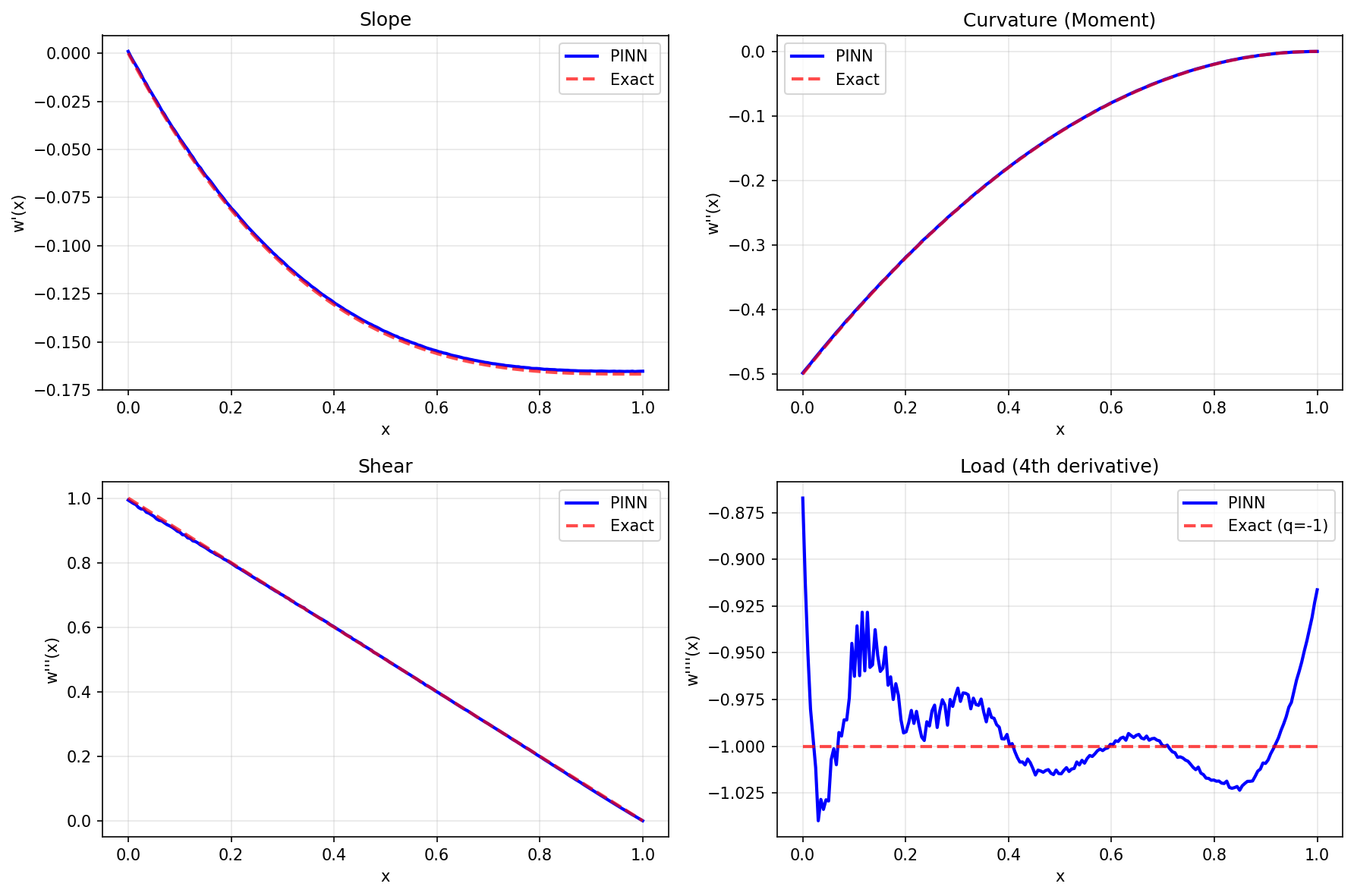
Physical Interpretation¶

Deflection \(w(x)\): Vertical displacement of beam centerline
Slope \(w'(x)\): Rotation angle of beam cross-section
Curvature \(w''(x)\): Related to bending moment \(M = EI \cdot w''\)
Shear \(w'''(x)\): Related to shear force \(V = EI \cdot w'''\)

Implementation¶

Step 1: Imports and Configuration¶

import jax
import jax.numpy as jnp
import optax
from flax import nnx

Terminal Output:

======================================================================
Opifex Example: Euler-Bernoulli Beam PINN
======================================================================
JAX backend: gpu
JAX devices: [CudaDevice(id=0)]

Euler-Bernoulli beam: EI * d^4w/dx^4 = q
  Load: q = -1.0
Domain: x in [0.0, 1.0]
Collocation: 100 domain, 10 boundary
Network: [1] + [20, 20, 20] + [1]
Training: 15000 epochs @ lr=0.001

Step 2: Define the Problem¶

Q = -1.0  # Distributed load (negative = downward)
X_MIN, X_MAX = 0.0, 1.0

def exact_solution(x):
    """Exact solution for cantilever beam with uniform load."""
    return -(x**4) / 24 + (x**3) / 6 - (x**2) / 4

def exact_derivative(x):
    """First derivative: w'(x)."""
    return -(x**3) / 6 + (x**2) / 2 - x / 2

Terminal Output:

Cantilever beam (fixed at x=0, free at x=1):
  w(0) = 0      (deflection)
  w'(0) = 0     (slope)
  w''(1) = 0    (moment)
  w'''(1) = 0   (shear)
  q = -1.0      (uniform load)
  Solution: w = -x^4/24 + x^3/6 - x^2/4

Step 3: Create the PINN¶

class EulerBeamPINN(nnx.Module):
    def __init__(self, hidden_dims: list[int], *, rngs: nnx.Rngs):
        super().__init__()
        layers = []
        in_features = 1  # x only (no time)

        for hidden_dim in hidden_dims:
            layers.append(nnx.Linear(in_features, hidden_dim, rngs=rngs))
            in_features = hidden_dim

        layers.append(nnx.Linear(in_features, 1, rngs=rngs))
        self.layers = nnx.List(layers)

    def __call__(self, x: jax.Array) -> jax.Array:
        h = x
        for layer in self.layers[:-1]:
            h = jnp.tanh(layer(h))
        return self.layers[-1](h)

pinn = EulerBeamPINN(hidden_dims=[20, 20, 20], rngs=nnx.Rngs(42))

Terminal Output:

Creating PINN model...
PINN parameters: 901

Step 4: Generate Collocation Points¶

key = jax.random.PRNGKey(42)

# Domain interior points
x_domain = jax.random.uniform(key, (N_DOMAIN,), minval=X_MIN, maxval=X_MAX)
x_domain = x_domain.reshape(-1, 1)

# Boundary points
x_left = jnp.zeros((N_BOUNDARY // 2, 1))   # x = 0 (fixed end)
x_right = jnp.ones((N_BOUNDARY // 2, 1))   # x = 1 (free end)

Terminal Output:

Generating collocation points...
Domain points: (100, 1)
Left BC points: (5, 1)
Right BC points: (5, 1)

Step 5: Fourth Derivative Computation¶

The key challenge is computing the 4^th derivative using nested jax.grad calls:

def compute_derivatives(pinn, x):
    """Compute w, w', w'', w''', w'''' at given points."""

    def w_scalar(x_single):
        return pinn(x_single.reshape(1, 1)).squeeze()

    def derivatives_single(x_single):
        w = w_scalar(x_single)

        # w' = dw/dx
        w_x = jax.grad(w_scalar)(x_single)[0]

        # w'' = d^2w/dx^2
        def w_x_fn(xs):
            return jax.grad(w_scalar)(xs)[0]
        w_xx = jax.grad(w_x_fn)(x_single)[0]

        # w''' = d^3w/dx^3
        def w_xx_fn(xs):
            def w_x_inner(xs2):
                return jax.grad(w_scalar)(xs2)[0]
            return jax.grad(w_x_inner)(xs)[0]
        w_xxx = jax.grad(w_xx_fn)(x_single)[0]

        # w'''' = d^4w/dx^4
        def w_xxx_fn(xs):
            def w_xx_inner(xs2):
                def w_x_inner2(xs3):
                    return jax.grad(w_scalar)(xs3)[0]
                return jax.grad(w_x_inner2)(xs2)[0]
            return jax.grad(w_xx_inner)(xs)[0]
        w_xxxx = jax.grad(w_xxx_fn)(x_single)[0]

        return w, w_x, w_xx, w_xxx, w_xxxx

    return jax.vmap(derivatives_single)(x)

Step 6: Define Physics-Informed Loss¶

def pde_loss(pinn, x):
    """PDE loss: w'''' + 1 = 0 (since q=-1 and EI=1)."""
    _, _, _, _, w_xxxx = compute_derivatives(pinn, x)
    residual = w_xxxx - Q  # w'''' = q = -1
    return jnp.mean(residual**2)

def bc_loss(pinn, x_left, x_right):
    """Boundary condition losses for cantilever beam."""
    # Left BC: w(0) = 0, w'(0) = 0
    w_l, w_x_l, _, _, _ = compute_derivatives(pinn, x_left)
    loss_w0 = jnp.mean(w_l**2)
    loss_wx0 = jnp.mean(w_x_l**2)

    # Right BC: w''(1) = 0, w'''(1) = 0
    _, _, w_xx_r, w_xxx_r, _ = compute_derivatives(pinn, x_right)
    loss_wxx1 = jnp.mean(w_xx_r**2)
    loss_wxxx1 = jnp.mean(w_xxx_r**2)

    return loss_w0 + loss_wx0 + loss_wxx1 + loss_wxxx1

def total_loss(pinn, x_dom, x_left, x_right, lambda_bc=100.0):
    """Total loss = PDE + weighted BC."""
    loss_pde = pde_loss(pinn, x_dom)
    loss_bc = bc_loss(pinn, x_left, x_right)
    return loss_pde + lambda_bc * loss_bc

Step 7: Training¶

opt = nnx.Optimizer(pinn, optax.adam(LEARNING_RATE), wrt=nnx.Param)

@nnx.jit
def train_step(pinn, opt, x_dom, x_left, x_right):
    def loss_fn(model):
        return total_loss(model, x_dom, x_left, x_right)

    loss, grads = nnx.value_and_grad(loss_fn)(pinn)
    opt.update(pinn, grads)
    return loss

for epoch in range(EPOCHS):
    loss = train_step(pinn, opt, x_domain, x_left, x_right)

Terminal Output:

Training PINN...
  Epoch     1/15000: loss=2.477272e+02
  Epoch  3000/15000: loss=2.196092e-02
  Epoch  6000/15000: loss=2.239256e-03
  Epoch  9000/15000: loss=1.150323e-03
  Epoch 12000/15000: loss=8.906908e-03
  Epoch 15000/15000: loss=2.925966e-04
Final loss: 2.925966e-04

Step 8: Evaluation¶

Terminal Output:

Evaluating PINN...
Relative L2 error:   9.822021e-03
Maximum point error: 1.229844e-03
Mean point error:    4.862132e-04

Boundary condition errors:
  w(0) = -5.951524e-05 (should be 0)
  w'(0) = 1.018226e-03 (should be 0)
  w''(1) = -1.121461e-04 (should be 0)
  w'''(1) = 6.520748e-05 (should be 0)

Visualization¶

Euler Beam Solution

Derivatives Analysis

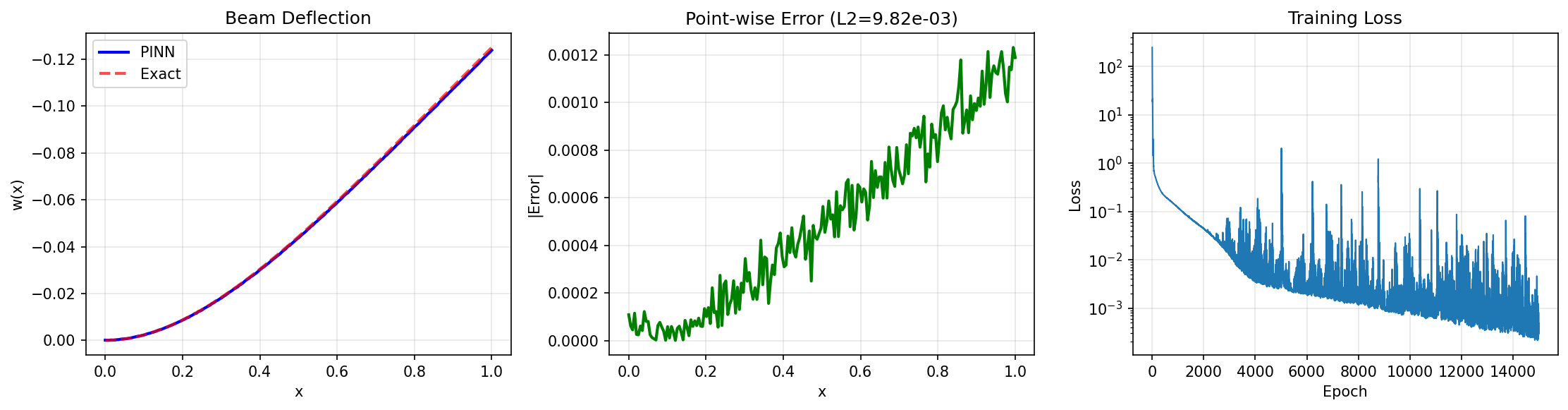
Results Summary¶

Metric	Value
Final Loss	2.93e-04
Relative L2 Error	0.98%
Maximum Error	1.23e-03
BC w(0)	-5.95e-05
BC w'(0)	1.02e-03
BC w''(1)	-1.12e-04
BC w'''(1)	6.52e-05
Parameters	901
Training Epochs	15,000

Next Steps¶

Experiments to Try¶

Hard constraints: Implement hard BC for w(0)=0 and w'(0)=0
Variable load: Use non-uniform q(x) like triangular or sinusoidal
Simply supported: Change BCs to w(0)=w(1)=0, w''(0)=w''(1)=0
2D plate: Extend to biharmonic equation for plate bending

Example	Level	What You'll Learn
Poisson Equation	Beginner	2^nd-order elliptic PDE
Helmholtz Equation	Intermediate	2^nd-order with wavenumber
Wave Equation	Intermediate	2^nd-order in time

Troubleshooting¶

Issue	Solution
BC not satisfied	Increase lambda_bc weight or training epochs
Derivative noise	Use more hidden layers or wider network
Slow 4^th derivative	Pre-compile with `jax.jit` outside training loop
Loss plateaus	Try learning rate scheduling or L-BFGS refinement

Euler-Bernoulli Beam PINN¶

Overview¶

What You'll Learn¶

Coming from DeepXDE?¶

Files¶

Quick Start¶

Run the Python Script¶

Run the Jupyter Notebook¶

Core Concepts¶

Euler-Bernoulli Beam Equation¶

Cantilever Beam Boundary Conditions¶

Physical Interpretation¶

Implementation¶

Step 1: Imports and Configuration¶

Step 2: Define the Problem¶

Step 3: Create the PINN¶

Step 4: Generate Collocation Points¶

Step 5: Fourth Derivative Computation¶

Step 6: Define Physics-Informed Loss¶

Step 7: Training¶

Step 8: Evaluation¶

Visualization¶

Results Summary¶

Next Steps¶

Experiments to Try¶

Related Examples¶

Troubleshooting¶