XPINN: Extended PINN on Viscous Burgers Equation

Filename Note

The filename xpinn-helmholtz is a historical artifact. This example solves the viscous Burgers equation, not the Helmholtz equation.

Metadata	Value
Level	Intermediate
Runtime	~2 min (GPU) / ~12 min (CPU)
Prerequisites	JAX, Flax NNX, PDEs
Format	Python + Jupyter
Memory	~400 MB RAM

Overview

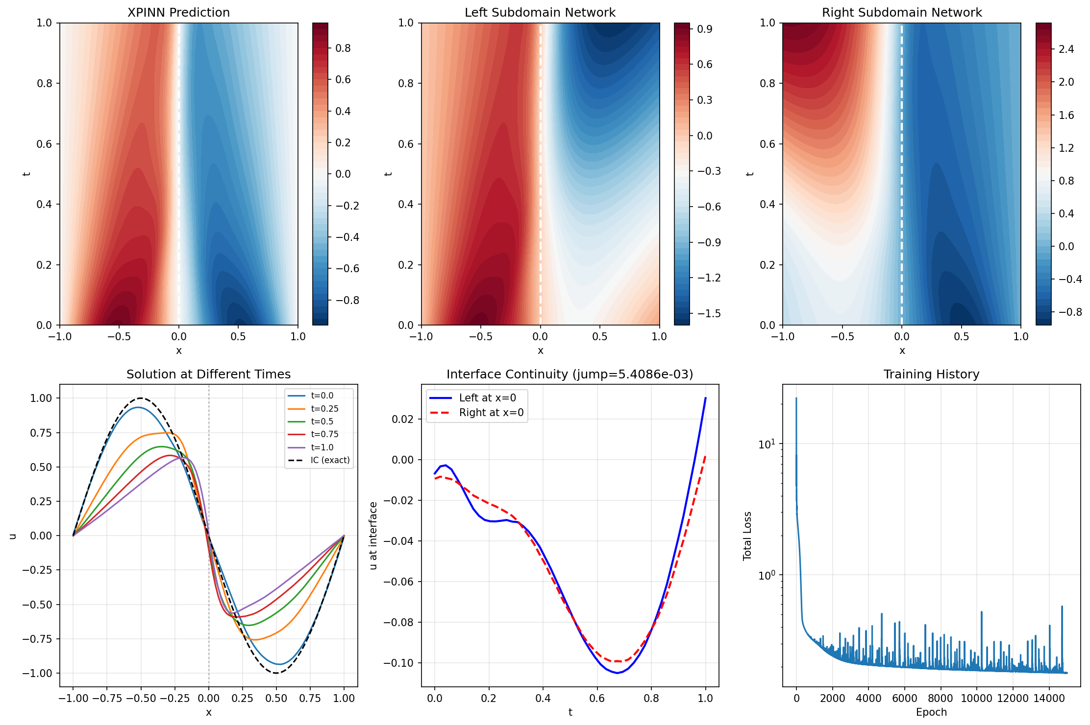
This example demonstrates solving the 1D viscous Burgers equation using XPINN (Extended Physics-Informed Neural Network). XPINNs use non-overlapping subdomains with explicit interface conditions for continuity and flux matching.

Unlike FBPINNs which use smooth window blending, XPINNs enforce interface conditions through additional loss terms. This makes XPINNs suitable for problems where sharp interfaces or discontinuities need to be captured.

What You'll Learn

1. Understand the XPINN architecture with non-overlapping subdomains
2. Implement interface continuity and flux matching conditions
3. Configure loss weights for interface enforcement
4. Use Opifex's XPINN class for domain decomposition
5. Visualize interface discontinuity and solution quality

Coming from XPINNs Literature?

XPINNs (Literature)	Opifex (JAX)
Separate networks per subdomain	XPINN class with SubdomainNetwork list
Interface continuity loss	model.compute_continuity_loss()
Flux matching loss	model.compute_flux_loss()
Weighted loss combination	XPINNConfig(continuity_weight=..., flux_weight=...)

Key differences:

1. Built-in methods: Interface losses computed via class methods
2. JIT-compatible: All interface computations are JAX-compatible
3. Configurable weights: Easy weight adjustment via config

Files

• Python Script: examples/domain-decomposition/xpinn_helmholtz.py
• Jupyter Notebook: examples/domain-decomposition/xpinn_helmholtz.ipynb

Quick Start

Run the Python Script

source activate.sh && python examples/domain-decomposition/xpinn_helmholtz.py

Run the Jupyter Notebook

jupyter lab examples/domain-decomposition/xpinn_helmholtz.ipynb

Core Concepts

XPINN Architecture

XPINNs decompose the domain into non-overlapping subdomains:

\[\Omega = \Omega_1 \cup \Omega_2 \cup \ldots \cup \Omega_N\]

At interfaces, we enforce: - Continuity: \(u_{left} = u_{right}\) - Flux matching: \(\frac{\partial u}{\partial n}_{left} = \frac{\partial u}{\partial n}_{right}\)

Component	This Example
Domain	\(x \in [-1, 1]\), \(t \in [0, 1]\)
Subdomains	2 (split at \(x = 0\))
Interface	Vertical line at \(x = 0\)
PDE	Viscous Burgers equation
Viscosity	\(\nu = 0.01/\pi\)

Viscous Burgers Equation

\[\frac{\partial u}{\partial t} + u \frac{\partial u}{\partial x} = \nu \frac{\partial^2 u}{\partial x^2}\]

With: - IC: \(u(x, 0) = -\sin(\pi x)\) - BC: \(u(-1, t) = u(1, t) = 0\)

Implementation

Step 1: Imports and Configuration

from opifex.neural.pinns.domain_decomposition import (
    Interface,
    Subdomain,
    XPINN,
    XPINNConfig,
)

Terminal Output:

======================================================================
Opifex Example: XPINN on 1D Viscous Burgers Equation
======================================================================
JAX backend: gpu
JAX devices: [CudaDevice(id=0)]

Viscous Burgers: du/dt + u*du/dx = nu*d^2u/dx^2
  Viscosity: nu = 0.01/pi ~ 0.003183
Domain: x in [-1.0, 1.0], t in [0.0, 1.0]
Subdomains: 2
Network per subdomain: [2] + [40, 40, 40] + [1]
Training: 15000 epochs @ lr=0.001

Step 2: Define Subdomains and Interfaces

# Non-overlapping subdomains
subdomains = [
    Subdomain(id=0, bounds=jnp.array([[-1.0, 0.0], [0.0, 1.0]])),  # Left
    Subdomain(id=1, bounds=jnp.array([[0.0, 1.0], [0.0, 1.0]])),   # Right
]

# Interface at x = 0
interface_points = jnp.column_stack([
    jnp.zeros(N_INTERFACE),
    jnp.linspace(0.0, 1.0, N_INTERFACE),
])

interfaces = [
    Interface(
        subdomain_ids=(0, 1),
        points=interface_points,
        normal=jnp.array([1.0, 0.0]),
    )
]

Terminal Output:

Creating XPINN model...
Total XPINN parameters: 6882
Parameters per subdomain: ~3441

Step 3: Configure XPINN

xpinn_config = XPINNConfig(
    continuity_weight=10.0,  # u_left = u_right
    flux_weight=10.0,        # du/dx_left = du/dx_right
    residual_weight=1.0,     # PDE residual
)

model = XPINN(
    input_dim=2, output_dim=1,
    subdomains=subdomains,
    interfaces=interfaces,
    hidden_dims=[40, 40, 40],
    config=xpinn_config,
    rngs=nnx.Rngs(42),
)

Step 4: Training with Interface Conditions

Terminal Output:

Training XPINN...
  Epoch     1/15000: loss=2.217746e+01, continuity=1.131944e-02, flux=5.758483e-01
  Epoch  3000/15000: loss=2.154962e-01, continuity=8.435045e-05, flux=5.011343e-04
  Epoch  6000/15000: loss=2.030331e-01, continuity=1.473404e-04, flux=7.426925e-04
  Epoch  9000/15000: loss=1.890347e-01, continuity=7.456433e-05, flux=2.159171e-05
  Epoch 12000/15000: loss=1.837308e-01, continuity=8.042133e-05, flux=4.365924e-05
  Epoch 15000/15000: loss=1.795815e-01, continuity=5.910662e-05, flux=1.106780e-04
Final loss: 1.795815e-01

Step 5: Evaluation

Terminal Output:

Evaluating XPINN...
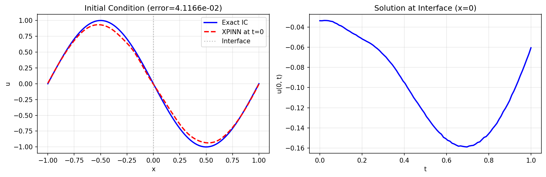
IC error (mean abs):     4.116559e-02
BC error (mean abs):     1.945176e-03
Interface jump:          5.408616e-03

Visualization

Results Summary

Metric	Value
Final Loss	0.18
IC Error	4.12e-02
BC Error	1.95e-03
Interface Jump	5.41e-03
Continuity Loss	5.91e-05
Flux Loss	1.11e-04
Parameters	6,882
Training Epochs	15,000

Next Steps

Experiments to Try

1. More subdomains: Split into 4 or 8 subdomains
2. Higher viscosity: Try \(\nu = 0.1\) for smoother solutions
3. Longer time: Extend to \(t \in [0, 2]\) to see shock formation
4. Residual averaging: Enable average_residual_weight for interface

Related Examples

Example	Level	What You'll Learn
FBPINN on Harmonic Oscillator	Intermediate	Overlapping subdomains
CPINN on Advection	Intermediate	Flux conservation
Burgers PINN	Intermediate	Single-domain PINN

API Reference

• XPINN: XPINN class with interface conditions
• XPINNConfig: Configuration (weights for losses)
• Interface: Interface definition with points and normal
• compute_continuity_loss(): Solution continuity at interfaces
• compute_flux_loss(): Gradient continuity at interfaces

Troubleshooting

Issue	Solution
Large interface jump	Increase continuity_weight
Flux discontinuity	Increase flux_weight
Solution mismatch at t=0	Check IC loss weighting
Slow convergence	Adjust interface loss weights