DISCO Convolutions: Discretisation-Invariant Convolution on Arbitrary Point Sets

Metadata	Value
Level	Advanced
Runtime	~30 s (GPU) / ~2 min (CPU)
Prerequisites	JAX, Flax NNX, neural operators, quadrature basics
Format	Python + Jupyter
Memory	~0.5 GB

Overview

A standard convolution has a fixed pixel kernel: its receptive field shrinks as the grid refines, and it cannot be applied to non-grid (scattered) data at all. A discrete-continuous (DISCO) convolution (Ocampo, Price & McEwen 2023, arXiv:2209.13603 — the algorithm behind NVIDIA's torch_harmonics and spherical neural operators) instead parameterises the kernel as a continuous function kappa(r) = Σ_k w_k φ_k(r) and evaluates the convolution as a quadrature against the input samples:

\[(\kappa * f)(x_o) \approx \sum_i q_i\, \kappa(x_o - x_i)\, f(x_i).\]

Because the kernel lives in physical coordinates (not pixels) and the sum is a quadrature, the operator is discretisation-aware: the same learned kernel transfers across grid resolutions, and it works on irregular point sets. This example demonstrates both with measurements.

The radial basis reuses opifex's PiecewiseLinearBasis (the torch_harmonics filter basis), and the filter is normalised per output point (a partition of unity) as in the reference.

What You'll Learn

1. Build a DiscreteContinuousConv2d over arbitrary input/output point sets
2. Measure discretisation invariance: the same kernel on a finer grid gives a consistent result
3. Apply the same operator to an irregular (scattered) point cloud — impossible for a pixel conv

Files

• Python Script: examples/layers/disco_convolutions_example.py
• Jupyter Notebook: examples/layers/disco_convolutions_example.ipynb

Quick Start

source activate.sh && python examples/layers/disco_convolutions_example.py

Coming from neuraloperator / torch_harmonics?

neuraloperator / torch_harmonics	Opifex
DiscreteContinuousConv2d(in_channels, out_channels, grid_in, grid_out, quadrature_weights, kernel_shape)	DiscreteContinuousConv2d(in_channels, out_channels, in_coords, out_coords, quad_weights, num_basis=, radius=, rngs=)
PiecewiseLinearFilterBasis	opifex.neural.equivariant.PiecewiseLinearBasis

The geometry (input/output positions and quadrature weights) is fixed at construction so the normalised filter is precomputed once; the learnable parameters are the per-basis channel-mixing weights, independent of the geometry — which is exactly what lets the same kernel transfer to a new grid.

Core Concept

The convolution factorises into a fixed geometric filter and learnable channel weights:

out[b, o, d] = Σ_{i, k}  psi[o, i, k] · x[b, i, c] · weight[k, c, d]
                         └── geometry ──┘            └── learned ──┘

psi[o, i, k] = q_i · φ_k(|x_o − x_i|),  normalised so  Σ_i psi[o, i, k] = 1

φ_k are the piecewise-linear radial hats; q_i are quadrature weights (the measure each sample represents). The per-output normalisation (torch_harmonics's _normalize_convolution_filter_matrix) is the partition of unity that gives consistent magnitude across discretisations.

Results

1. Discretisation invariance (convergence)

The same continuous kernel is applied to a smooth field sampled on grids of increasing resolution, read out at a fixed set of query points. The output converges as the grid refines:

Terminal Output:

Discretisation invariance (same continuous kernel, refining the input grid):
------------------------------------------------------------------------
  output @ query points (24x24): [-0.0824 -0.0115 -0.0501  0.0297  0.0907]
  output @ query points (96x96): [-0.0791 -0.0115 -0.0506  0.0336  0.0813]
  relative change 24->96: 0.0826
  relative change 48->96: 0.0112  (halves as the grid refines: convergent)

The relative change drops from 0.083 (24×24 vs 96×96) to 0.011 (48×48 vs 96×96) — roughly a 7× reduction as the grid refines toward the continuum. A standard pixel convolution has no such guarantee: its kernel is tied to the grid spacing, so refining the grid changes the operator.

2. Irregular (scattered) point set

Irregular (scattered) point set:
------------------------------------------------------------------------
  500 scattered points, same kernel -> output [-0.0819 -0.0176 -0.0826  0.0094  0.1003]
  agreement with the 96x96 grid result: relative diff 0.3479
  (a standard pixel convolution cannot be applied to scattered points at all)

The same operator runs directly on 500 randomly scattered points using Monte-Carlo quadrature weights — something a pixel convolution cannot do at all. The result approximates the grid convolution (relative diff 0.35 with only 500 random points; Monte-Carlo quadrature converges as 1/sqrt(N), so more points or a proper quadrature rule tighten the agreement).

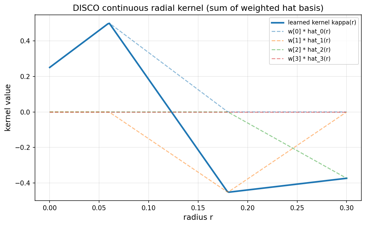
3. The learned continuous kernel

The kernel is a weighted sum of piecewise-linear radial hat functions — a genuinely continuous profile, not a pixel stencil:

Results Summary

Property	Measurement	What it shows
Discretisation invariance	rel. change 0.083 (24→96) → 0.011 (48→96)	Same kernel converges as grid refines
Irregular-grid capability	500 scattered points, rel. diff 0.35 vs grid	Runs on non-grid data (pixel conv cannot)
Continuous kernel	Σ_k w_k φ_k(r) over 4 hat bases	Kernel in physical coords, not pixels

Next Steps

Experiments to Try

1. Increase the scattered-point count and watch the irregular-grid agreement improve (1/sqrt(N)).
2. Vary num_basis and radius to trade kernel expressivity against support.
3. Stack DiscreteContinuousConv2d layers into an encoder on an irregular mesh.

Related Examples

Example	Level	What You'll Learn
Grid Embeddings	Beginner	Spatial coordinate injection for neural operators
Spectral Normalization	Intermediate	Lipschitz control for stable deep operators
Fourier Continuation	Intermediate	Boundary handling for spectral methods

API Reference

• DiscreteContinuousConv2d — general DISCO convolution layer
• build_disco_filter — the normalised quadrature filter psi[o, i, k]
• regular_grid — uniform grid coordinates and quadrature weights
• PiecewiseLinearBasis — the continuous radial basis