Grid Embeddings: Why Positional Coordinates Matter for Neural Operators
| Metadata | Value |
|---|---|
| Level | Intermediate |
| Runtime | ~3 min (GPU) / ~12 min (CPU) |
| Prerequisites | JAX, Flax NNX, FNO on Darcy |
| Format | Python + Jupyter |
| Memory | ~1 GB |
Overview
A Fourier Neural Operator sees only channel values at grid points — it has no intrinsic
notion of where each point sits in the domain. GridEmbedding2D
injects the spatial coordinates as extra input channels, giving the operator positional
awareness. This is standard practice in neural-operator libraries (it is on by default in
neuraloperator), but how much does it actually help?
This example answers that with a controlled ablation: two otherwise-identical FNOs are
trained on Darcy flow — one with GridEmbedding2D, one without — and we measure the difference
in test accuracy. Everything else (Fourier modes, width, depth, optimiser, data, random seed) is
held fixed, so the gap is attributable to the positional encoding alone.
What You'll Learn
- Compose
GridEmbedding2Dwith aFourierNeuralOperator - Quantify grid embedding's effect on test error (relative L2) with a clean ablation
- Visualise the coordinate channels the embedding appends to the input
- Understand why a boundary-value problem (fixed zero boundary) rewards positional awareness
Files
- Python Script:
examples/layers/grid_embeddings_example.py - Jupyter Notebook:
examples/layers/grid_embeddings_example.ipynb
Quick Start
Coming from neuraloperator (PyTorch)?
| neuraloperator | Opifex |
|---|---|
GridEmbeddingND(in_channels, dim, grid_boundaries) |
GridEmbedding2D(in_channels=, grid_boundaries=) / GridEmbeddingND(...) |
FNO(..., positional_embedding='grid') (default on) |
compose GridEmbedding2D then FourierNeuralOperator explicitly |
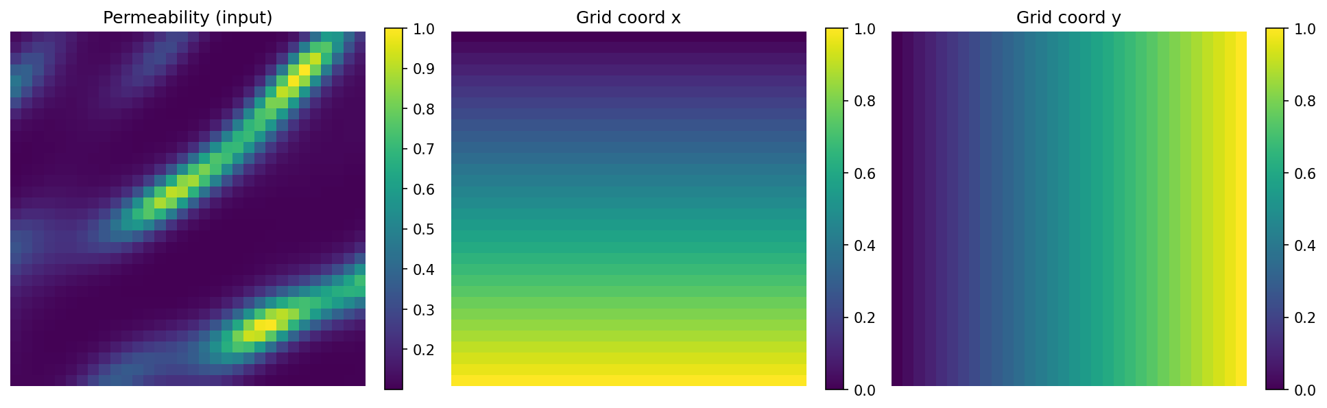
Key Concept: the coordinate channels
GridEmbedding2D takes a channels-last field and appends two channels holding the normalised
x and y coordinates of every grid point, turning a 1-channel permeability field into a
3-channel input. Those coordinate channels are constant across samples but vary smoothly across
space, so the operator can condition its response on position — essential when the boundary
condition pins the solution at the domain edge.
The Ablation
Both models are the same FNO (modes=12, hidden_channels=32, num_layers=4, domain_padding=0.25);
the only difference is the embedding:
class FNOWithGridEmbedding(nnx.Module):
    def __init__(self, modes, hidden_channels, num_layers, *, rngs):
        self.grid_embedding = GridEmbedding2D(
            in_channels=1, grid_boundaries=[[0.0, 1.0], [0.0, 1.0]]
        )
        self.fno = FourierNeuralOperator(
            in_channels=self.grid_embedding.out_channels,  # 3
            out_channels=1, hidden_channels=hidden_channels,
            modes=modes, num_layers=num_layers, domain_padding=0.25, rngs=rngs,
        )

    def __call__(self, x):
        x_hwc = jnp.moveaxis(x, 1, -1)
        x_embedded = self.grid_embedding(x_hwc)
        return self.fno(jnp.moveaxis(x_embedded, -1, 1))
Both are trained identically (1000 samples, 120 epochs, relative_l2 loss, AdamW) via
Trainer.fit().
Results
Terminal Output:
========================================================================
RESULTS — test relative L2 error (lower is better)
========================================================================
  FNO (no grid embedding):  0.0136
  FNO + GridEmbedding2D:    0.0102
  Grid embedding reduces the relative-L2 error by 25% on this boundary-value problem.
| Model | Test relative L2 |
|---|---|
| FNO (no grid embedding) | 0.0136 |
FNO + GridEmbedding2D |
0.0102 |
Adding the two coordinate channels — a negligible parameter increase — cuts the relative-L2 error by ~25%. On Darcy flow the solution is pinned to zero on the boundary, so knowing where a point is relative to the boundary is genuinely informative; the grid embedding supplies exactly that signal.
Scope
This is an in-distribution ablation at a fixed resolution. Grid coordinates are continuous and so are resolution-independent, but cross-resolution generalisation on Darcy also depends on the input distribution matching across discretisations, which is a separate concern not measured here.
Next Steps
Experiments to Try
- Vary
grid_boundariesto match a non-unit domain and confirm the embedding rescales. - Swap
GridEmbedding2DforSinusoidalEmbedding(Transformer-style frequency encoding) and compare. - Repeat the ablation on a periodic problem (e.g. Burgers) where positional awareness matters less.
Related Examples
- FNO on Darcy Flow — the full FNO recipe this builds on.
- Spectral Normalization — another neural-operator building block.
API Reference
GridEmbedding2D— 2D coordinate embeddingFourierNeuralOperator— the FNO modelTrainer— training orchestration