Burgers Equation PINN¶

Metadata	Value
Level	Intermediate
Runtime	~3 min (GPU) / ~10 min (CPU)
Prerequisites	JAX, Flax NNX, calculus basics
Format	Python + Jupyter
Memory	~500 MB RAM

Overview¶

This tutorial demonstrates solving the 1D viscous Burgers equation using a Physics-Informed Neural Network (PINN). The Burgers equation is a fundamental nonlinear PDE that serves as a simplified model for fluid dynamics and shock wave formation.

The Burgers equation combines nonlinear advection with viscous diffusion, making it an important testbed for numerical methods. PINNs can capture sharp gradients and shock-like behavior without explicit shock-capturing schemes required by traditional methods.

What You'll Learn¶

Implement a PINN for time-dependent nonlinear PDEs
Sample collocation points for domain, boundary, and initial conditions
Compute gradients using JAX autodiff (first and second derivatives)
Balance PDE residual, IC, and BC losses with appropriate weights
Visualize spatiotemporal solutions and solution evolution

Coming from DeepXDE?¶

If you are familiar with the DeepXDE library:

DeepXDE	Opifex (JAX)
`dde.geometry.GeometryXTime(geom, timedomain)`	`jax.random.uniform(key, (N, 2))` for (x, t)
`dde.grad.jacobian(y, x, i=0, j=1)`	`jax.grad(u_fn, argnums=1)(x, t)` for u_t
`dde.icbc.IC(geom, func, lambda_fun)`	Manual initial condition sampling + loss term
`dde.icbc.DirichletBC(geom, func, boundary)`	Manual boundary sampling + loss term
`dde.data.TimePDE(geom, pde, ic, bc, num_domain)`	Explicit collocation arrays
`model.compile("adam", lr=1e-3)`	`nnx.Optimizer(pinn, optax.adam(lr), wrt=nnx.Param)`
`model.train(iterations=15000)`	Custom training loop with `@nnx.jit`

Key differences:

Pure JAX autodiff: Use jax.grad directly instead of custom gradient APIs
Explicit collocation: Collocation points are simple JAX arrays
Separate IC/BC sampling: Initial and boundary conditions are sampled separately
JIT compilation: Entire training step is XLA-compiled for GPU acceleration

Files¶

Python Script: examples/pinns/burgers.py
Jupyter Notebook: examples/pinns/burgers.ipynb

Quick Start¶

Run the Python Script¶

source activate.sh && python examples/pinns/burgers.py

Run the Jupyter Notebook¶

jupyter lab examples/pinns/burgers.ipynb

Core Concepts¶

Burgers Equation¶

The 1D viscous Burgers equation is a nonlinear parabolic PDE:

\[\frac{\partial u}{\partial t} + u \frac{\partial u}{\partial x} = \nu \frac{\partial^2 u}{\partial x^2}\]

where \(\nu\) is the kinematic viscosity (diffusion coefficient).

Component	This Example
Domain	\(x \in [-1, 1]\), \(t \in [0, 0.99]\)
Viscosity	\(\nu = 0.01/\pi \approx 0.003183\)
Initial condition	\(u(x, 0) = -\sin(\pi x)\)
Boundary conditions	\(u(\pm 1, t) = 0\) (Dirichlet)

Physical Interpretation¶

The Burgers equation models:

Nonlinear advection (\(u \cdot u_x\)): Wave steepening and shock formation
Viscous diffusion (\(\nu \cdot u_{xx}\)): Smoothing that prevents discontinuities

At low viscosity, the solution develops steep gradients. This example uses moderate viscosity where the solution remains smooth but shows characteristic nonlinear behavior.

PINN Loss Components¶

graph TB
    subgraph Input["Collocation Points"]
        A["Domain Points<br/>(x, t) in Ω"]
        B["Initial Points<br/>(x, 0)"]
        C["Boundary Points<br/>(±1, t)"]
    end

    subgraph PINN["Neural Network u_θ(x, t)"]
        D["Linear + tanh<br/>20 units"]
        E["Linear + tanh<br/>20 units"]
        F["Linear + tanh<br/>20 units"]
        G["Linear<br/>1 unit"]
    end

    subgraph Loss["Physics-Informed Loss"]
        H["PDE Residual<br/>|u_t + u·u_x - ν·u_xx|²"]
        I["IC Loss<br/>|u(x,0) - u₀(x)|²"]
        J["BC Loss<br/>|u(±1,t)|²"]
        K["Total Loss<br/>L_pde + λ_ic·L_ic + λ_bc·L_bc"]
    end

    A --> D --> E --> F --> G --> H
    B --> D
    C --> D
    G --> I
    G --> J
    H --> K
    I --> K
    J --> K

    style H fill:#e3f2fd,stroke:#1976d2
    style I fill:#e8f5e9,stroke:#388e3c
    style J fill:#fff3e0,stroke:#f57c00
    style K fill:#f3e5f5,stroke:#7b1fa2

Computing Derivatives¶

The PDE residual requires first and second derivatives:

def compute_pde_residual(pinn, x, t):
    def u_fn(x_single, t_single):
        xt = jnp.array([x_single, t_single])
        return pinn(xt.reshape(1, 2)).squeeze()

    def residual_single(x_single, t_single):
        # First derivatives
        u = u_fn(x_single, t_single)
        u_t = jax.grad(u_fn, argnums=1)(x_single, t_single)
        u_x = jax.grad(u_fn, argnums=0)(x_single, t_single)

        # Second derivative
        u_xx = jax.grad(lambda x: jax.grad(u_fn, argnums=0)(x, t_single))(x_single)

        # Burgers: u_t + u*u_x - nu*u_xx = 0
        return u_t + u * u_x - NU * u_xx

    return jax.vmap(residual_single)(x, t)

Implementation¶

Step 1: Imports and Configuration¶

import jax
import jax.numpy as jnp
import optax
from flax import nnx

Terminal Output:

======================================================================
Opifex Example: Burgers Equation PINN
======================================================================
JAX backend: gpu
JAX devices: [CudaDevice(id=0)]
Domain: x ∈ [-1.0, 1.0], t ∈ [0.0, 0.99]
Viscosity: nu = 0.003183
Collocation: 2540 domain, 80 boundary, 160 initial
Network: [2] + [20, 20, 20] + [1]
Training: 15000 epochs @ lr=0.001

Step 2: Define the Problem¶

# DeepXDE configuration
NU = 0.01 / jnp.pi  # Viscosity
X_MIN, X_MAX = -1.0, 1.0
T_MIN, T_MAX = 0.0, 0.99

# Collocation points (matching DeepXDE)
N_DOMAIN = 2540
N_BOUNDARY = 80
N_INITIAL = 160

def initial_condition(x):
    """Initial condition: u(x, 0) = -sin(πx)."""
    return -jnp.sin(jnp.pi * x)

Terminal Output:

Burgers equation: du/dt + u*du/dx = nu*d2u/dx2
Initial condition: u(x, 0) = -sin(πx)
Boundary conditions: u(±1, t) = 0

Step 3: Create the PINN¶

class BurgersPINN(nnx.Module):
    def __init__(self, hidden_dims: list[int], *, rngs: nnx.Rngs):
        layers = []
        in_features = 2  # (x, t)

        for hidden_dim in hidden_dims:
            layers.append(nnx.Linear(in_features, hidden_dim, rngs=rngs))
            in_features = hidden_dim

        layers.append(nnx.Linear(in_features, 1, rngs=rngs))
        self.layers = nnx.List(layers)

    def __call__(self, xt: jax.Array) -> jax.Array:
        h = xt
        for layer in self.layers[:-1]:
            h = jnp.tanh(layer(h))
        return self.layers[-1](h)

pinn = BurgersPINN(hidden_dims=[20, 20, 20], rngs=nnx.Rngs(42))

Terminal Output:

Creating PINN model...
PINN parameters: 921

Step 4: Generate Collocation Points¶

# Domain points (interior)
x_domain = jax.random.uniform(key1, (N_DOMAIN,), minval=X_MIN, maxval=X_MAX)
t_domain = jax.random.uniform(key2, (N_DOMAIN,), minval=T_MIN, maxval=T_MAX)

# Initial condition points (t = 0)
x_initial = jax.random.uniform(key3, (N_INITIAL,), minval=X_MIN, maxval=X_MAX)
t_initial = jnp.zeros(N_INITIAL)

# Boundary points (x = ±1)
t_boundary = jax.random.uniform(key4, (N_BOUNDARY,), minval=T_MIN, maxval=T_MAX)
x_boundary_left = jnp.full(N_BOUNDARY // 2, X_MIN)
x_boundary_right = jnp.full(N_BOUNDARY // 2, X_MAX)

Terminal Output:

Generating collocation points...
Domain points:   (2540, 2)
Boundary points: (80, 2)
Initial points:  (160, 2)

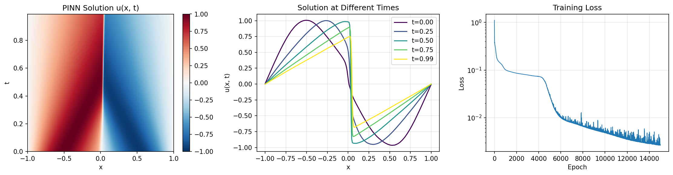
Step 5: Training¶

Terminal Output:

Training PINN...
  Epoch     1/15000: loss=1.109028e+00
  Epoch  3000/15000: loss=7.919201e-02
  Epoch  6000/15000: loss=1.014442e-02
  Epoch  9000/15000: loss=5.904152e-03
  Epoch 12000/15000: loss=3.557441e-03
  Epoch 15000/15000: loss=2.660285e-03
Final loss: 2.660285e-03

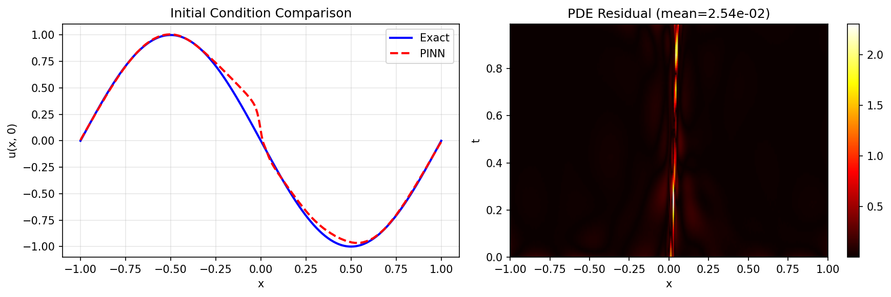
Step 6: Evaluation¶

Terminal Output:

Evaluating PINN...
Mean PDE residual: 2.539036e-02
Initial condition error: 3.055971e-02
Boundary condition error: 2.018995e-03

Visualization¶

Solution Evolution¶

Burgers Equation Solution

Analysis¶

Solution Analysis

Results Summary¶

Metric	Value
Final Loss	2.66e-03
Mean PDE Residual	2.54e-02
IC Error	3.06e-02
BC Error	2.02e-03
Parameters	921
Training Epochs	15,000

Next Steps¶

Experiments to Try¶

Higher viscosity: Try \(\nu = 0.1/\pi\) for smoother solutions
Lower viscosity: Try \(\nu = 0.001/\pi\) to see steeper gradients
Larger network: Use hidden_dims=[40, 40, 40, 40] for higher accuracy
More epochs: Train for 30,000+ epochs for better convergence
Adaptive weights: Implement loss balancing for IC/BC terms

Example	Level	What You'll Learn
Poisson Equation	Intermediate	Elliptic PDEs
Heat Equation	Intermediate	Simpler time-dependent PDE
FNO on Burgers	Intermediate	Data-driven alternative
PINO on Burgers	Advanced	Hybrid approach

API Reference¶

nnx.Linear - Linear layer
nnx.Optimizer - Optimizer wrapper
jax.grad - Gradient computation
jax.vmap - Vectorized mapping

Troubleshooting¶

Loss oscillates or diverges¶

Symptom: Training loss fluctuates wildly or increases.

Cause: Learning rate too high or poorly balanced loss terms.

Solution: Reduce learning rate or adjust loss weights:

# Lower learning rate
LEARNING_RATE = 5e-4

# Adjust loss weights
lambda_ic = 100.0  # Increase if IC not satisfied
lambda_bc = 100.0  # Increase if BCs not satisfied

Solution blows up at later times¶

Symptom: Solution looks good near t=0 but becomes incorrect at larger t.

Cause: Insufficient domain collocation points in later time region.

Solution: Use more domain points or time-stratified sampling:

# Stratified sampling in time
t_bins = jnp.linspace(T_MIN, T_MAX, 10)
points_per_bin = N_DOMAIN // 9
t_domain = jnp.concatenate([
    jax.random.uniform(key, (points_per_bin,), minval=t_bins[i], maxval=t_bins[i+1])
    for i, key in enumerate(jax.random.split(key, 9))
])

IC error much higher than PDE residual¶

Symptom: Initial condition has large error compared to PDE residual.

Cause: Network prioritizes minimizing PDE over satisfying IC.

Solution: Increase IC loss weight or use hard constraint:

# Hard BC/IC constraint (recommended)
def hard_constraint(pinn, xt):
    x, t = xt[:, 0], xt[:, 1]
    u_nn = pinn(xt).squeeze()
    # Multiply by t to enforce u(x,0) = 0, add IC
    return u_nn * t + (1 - t) * initial_condition(x)

Slow convergence¶

Symptom: Need many epochs (>50,000) to converge.

Cause: Network architecture not suited for solution structure.

Solution: Use tanh activation (smooth), deeper network, or Fourier features:

# Fourier feature encoding
def fourier_features(xt, scales=[1, 2, 4, 8]):
    features = [xt]
    for s in scales:
        features.append(jnp.sin(s * jnp.pi * xt))
        features.append(jnp.cos(s * jnp.pi * xt))
    return jnp.concatenate(features, axis=-1)

Comparison with DeepXDE¶

Both frameworks solve the same Burgers equation with identical network size ([2, 20, 20, 20, 1]) and training configuration (2540 domain points, 80 boundary, 160 initial condition points, 15000 Adam iterations).

Results from running on the same hardware:

Metric	Opifex (JAX)	DeepXDE (TensorFlow)
Final loss	2.66e-3	5.80e-3
Mean PDE residual	2.54e-2	3.23e-2
L2 relative error	--	0.291
BC error	2.02e-3	--
Parameters	921	921

Opifex achieves lower final loss (2.66e-3 vs 5.80e-3) and lower PDE residual (2.54e-2 vs 3.23e-2) with the same architecture and training budget.

Opifex advantages: JIT-compiled training loop, explicit PRNG control, composable JAX transforms (jax.grad, jax.vmap), hard constraint support.

Burgers Equation PINN¶

Overview¶

What You'll Learn¶

Coming from DeepXDE?¶

Files¶

Quick Start¶

Run the Python Script¶

Run the Jupyter Notebook¶

Core Concepts¶

Burgers Equation¶

Physical Interpretation¶

PINN Loss Components¶

Computing Derivatives¶

Implementation¶

Step 1: Imports and Configuration¶

Step 2: Define the Problem¶

Step 3: Create the PINN¶

Step 4: Generate Collocation Points¶

Step 5: Training¶

Step 6: Evaluation¶

Visualization¶

Solution Evolution¶

Analysis¶

Results Summary¶

Next Steps¶

Experiments to Try¶

Related Examples¶

API Reference¶

Troubleshooting¶

Loss oscillates or diverges¶

Solution blows up at later times¶

IC error much higher than PDE residual¶

Slow convergence¶

Comparison with DeepXDE¶