Meta-Optimization: MAML and Reptile for a Family of PDEs
| Metadata | Value |
|---|---|
| Level | Advanced |
| Runtime | ~3 min (GPU) / ~10 min (CPU) |
| Prerequisites | JAX, Flax NNX, PINNs, gradient-based meta-learning |
| Format | Python + Jupyter |
| Memory | ~1 GB |
Overview
Solving a family of PDEs that differ only in a parameter (here the Burgers viscosity nu) by
training a fresh physics-informed network (PINN) for each instance wastes the structure shared
across the family. Gradient-based meta-learning instead learns a single initialisation theta
such that a handful of ordinary gradient steps adapt it to any new nu — amortising the shared
physics into the starting point.
This example meta-learns that initialisation with opifex's maml_meta_train and
reptile_meta_train (the real algorithms — MAML, Finn et al. 2017,
arXiv:1703.03400; Reptile, Nichol et al. 2018,
arXiv:1803.02999), then measures few-shot adaptation on
held-out viscosities against training a fresh network from a random initialisation.
The Burgers PINN is expressed as a Task / TaskFamily (the same abstraction the
learned-optimiser stack uses), so the example only supplies the physics — the meta-learning comes
from the library.
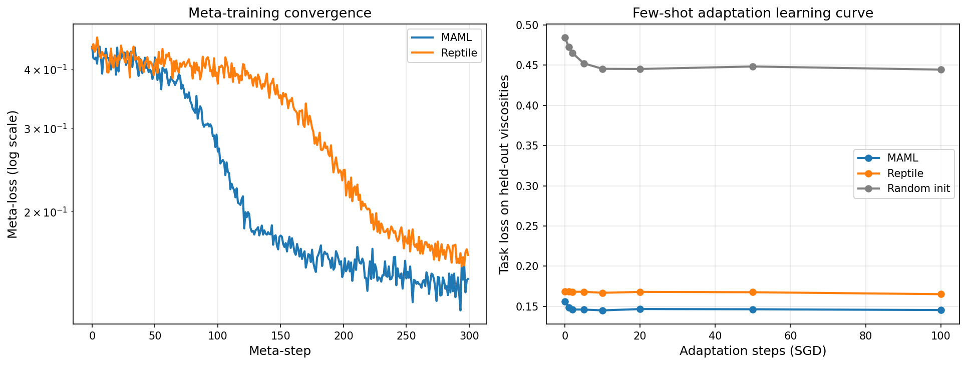
Key result: both meta-learned initialisations solve unseen viscosities zero-shot (MAML 0.156, Reptile 0.168 task loss) to a loss 65% below what a random initialisation reaches after 100 SGD adaptation steps (0.445).
What You'll Learn
- Express a PDE-solver family as an opifex
Task/TaskFamily - Meta-learn a PINN initialisation with
maml_meta_trainandreptile_meta_train - Measure few-shot
adapt-ation on unseen viscosities via the learning curve vs a from-scratch baseline
Files
- Python script:
examples/optimization/meta_optimization.py - Jupyter notebook:
examples/optimization/meta_optimization.ipynb
Quick Start
Core Concepts
Task / TaskFamily
The meta-trainers operate on a TaskFamily — a distribution over objectives. A BurgersTask is
one viscosity (init samples PINN parameters; loss is the physics-informed loss on freshly
sampled collocation points), and BurgersTaskFamily.sample draws a viscosity uniformly from
[NU_MIN, NU_MAX]. Parameters are a plain pytree of (weight, bias) tuples so the meta-trainers
can differentiate through inner adaptation.
@dataclass(frozen=True)
class BurgersTask(Task):
    nu: jax.Array

    def init(self, key):
        return init_pinn_params(key)

    def loss(self, params, key):
        xt_domain, xt_initial, u_initial, xt_boundary = sample_collocation(key)
        loss_pde = jnp.mean(burgers_residual(params, xt_domain, self.nu) ** 2)
        loss_ic = jnp.mean((pinn_forward(params, xt_initial).squeeze() - u_initial) ** 2)
        loss_bc = jnp.mean(pinn_forward(params, xt_boundary).squeeze() ** 2)
        return loss_pde + loss_ic + loss_bc
Task Distribution: Burgers Equation
The Burgers equation with varying viscosity ν:
- Low viscosity (ν → 0): sharp gradients, shock-like behaviour
- High viscosity: smooth, diffusion-dominated solutions
- Meta-learning: captures the common structure across the viscosity range
MAML vs Reptile
| Aspect | MAML | Reptile |
|---|---|---|
| Meta-objective | Post-adaptation (query) loss, differentiated through the inner steps (first_order=True here) |
Move theta towards each task's adapted parameters |
| Inner trajectory | Short (5 steps) | Longer (20 steps) — needed to move theta |
| Zero-shot loss (this run) | 0.156 | 0.168 |
Coming from Other Meta-Learning Frameworks?
| Framework | Opifex |
|---|---|
learn2learn / higher MAML |
maml_meta_train(task_family, init_params, key, ..., first_order=False) |
| Reptile implementations | reptile_meta_train(task_family, init_params, key, ...) |
| Inner-loop fine-tuning | adapt(task, init_params, key, inner_steps=, inner_lr=) |
| Task distribution | TaskFamily.sample(key) -> Task |
Implementation
Step 1: Meta-train both initialisations
from opifex.optimization.l2o.meta_learning import adapt, maml_meta_train, reptile_meta_train

family = BurgersTaskFamily()
init_params = init_pinn_params(init_key)  # shared starting point

maml_params, maml_curve = maml_meta_train(
    family, init_params, maml_key,
    num_outer_steps=300, num_tasks=8, inner_steps=5, inner_lr=0.01,
    meta_lr=1e-3, first_order=True,
)
reptile_params, reptile_curve = reptile_meta_train(
    family, init_params, reptile_key,
    num_outer_steps=300, num_tasks=8, inner_steps=20, inner_lr=0.01, meta_lr=0.3,
)
Terminal Output:
PINN architecture (2, 32, 32, 1)  (1,185 parameters)
Task family: Burgers viscosity ~ U[0.005, 0.05]

Meta-training MAML (first-order) for 300 steps...
Meta-training Reptile for 300 steps...
  MAML    meta-loss: 0.4461 -> 0.1442
  Reptile meta-loss: 0.4434 -> 0.1620
Step 2: Few-shot learning curve on held-out viscosities
For each held-out viscosity, adapt (plain SGD — the inner rule meta-training assumes) from each
initialisation and record the task loss after k steps:
def few_shot_loss(start, nu, key, steps):
    task = BurgersTask(nu=nu)
    adapted = adapt(task, start, key, inner_steps=steps, inner_lr=0.01)
    return float(task.loss(adapted, jax.random.fold_in(key, 7)))
Terminal Output:
Few-shot adaptation on 4 held-out viscosities
(SGD, inner_lr=0.01); task loss after k steps, averaged over viscosities:
------------------------------------------------------------------------
  steps         0        1        2        5       10       20       50      100
  MAML          0.1563   0.1484   0.1461   0.1460   0.1449   0.1466   0.1463   0.1453
  Reptile       0.1682   0.1681   0.1680   0.1681   0.1669   0.1679   0.1675   0.1651
  Random init   0.4846   0.4728   0.4652   0.4523   0.4455   0.4454   0.4484   0.4445

========================================================================
RESULTS — task loss on held-out viscosities (lower is better)
========================================================================
  MAML        zero-shot (0 steps): 0.1563
  Reptile     zero-shot (0 steps): 0.1682
  Random init zero-shot (0 steps): 0.4846
  Random init after 100 steps : 0.4445

  The best meta-init solves unseen viscosities ZERO-SHOT to a loss 65% below what a
  random init reaches after 100 SGD steps.
The meta-learned initialisations start in a low-loss basin and stay there; the random initialisation descends slowly with SGD and never catches up within 100 steps.
Visualization
Results Summary
| Initialisation | Zero-shot loss | Loss after 100 SGD steps |
|---|---|---|
| MAML | 0.156 | 0.145 |
| Reptile | 0.168 | 0.165 |
| Random | 0.485 | 0.445 |
Key Findings:
- Both meta-learned initialisations solve held-out viscosities zero-shot to a loss the random initialisation cannot reach in 100 SGD steps (a 65% reduction).
- MAML edges out Reptile here; Reptile needs a longer inner trajectory (20 vs 5 steps) to move its initialisation, after which it is competitive.
- The benefit is in the initialisation: the few-shot curves are nearly flat for the meta-inits because they already sit near the family's shared solution.
Next Steps
Experiments to Try
- Second-order MAML: pass
first_order=Falsetomaml_meta_train(more expensive — the PINN loss already uses second-order autodiff — but a tighter meta-gradient). - Wider viscosity range: widen
[NU_MIN, NU_MAX]and watch the random-init gap grow. - More meta-training: raise
META_STEPSandnum_tasksfor a lower zero-shot loss. - Different PDEs: define a new
TaskFamilyfor a heat- or wave-equation family.
Related Examples
- Learn-to-Optimize (L2O) — meta-learning an update rule (vs the initialisation meta-learned here)
API Reference
opifex.optimization.l2o.meta_learning.maml_meta_trainopifex.optimization.l2o.meta_learning.reptile_meta_trainopifex.optimization.l2o.meta_learning.adaptopifex.optimization.l2o.core.Task,opifex.optimization.l2o.core.TaskFamily
Troubleshooting
Reptile meta-loss barely moves
Reptile's update moves theta towards each task's adapted parameters; with too few inner steps the
adapted parameters barely differ from theta, so the move is tiny. Increase inner_steps (this
example uses 20) or raise meta_lr.
MAML init good for few steps but drifts over many
MAML optimises the initialisation for its inner step count. Evaluate few-shot quality near that budget, or meta-train with more inner steps to match the intended adaptation length.
Plain-SGD adaptation is unstable over many steps
PINNs trained with plain SGD plateau and can diverge at higher learning rates over long horizons. Keep the adaptation horizon short (the meta-learning win is in few steps) and the inner learning rate modest.