Neural Tangent Kernel (NTK) Analysis for PINNs
| Level | Runtime | Prerequisites | Format | Memory |
|---|---|---|---|---|
| Advanced | ~2 min | PINN basics, linear algebra | Tutorial | ~500 MB |
Overview
This example demonstrates how to use the Neural Tangent Kernel (NTK) to diagnose and understand PINN training dynamics. NTK analysis reveals spectral bias, predicts convergence rates, and identifies problematic modes.
SciML Context: Understanding why PINNs struggle with certain problems (high-frequency solutions, stiff PDEs) can be explained through NTK theory. The eigenvalue spectrum determines which solution modes are learned quickly vs slowly.
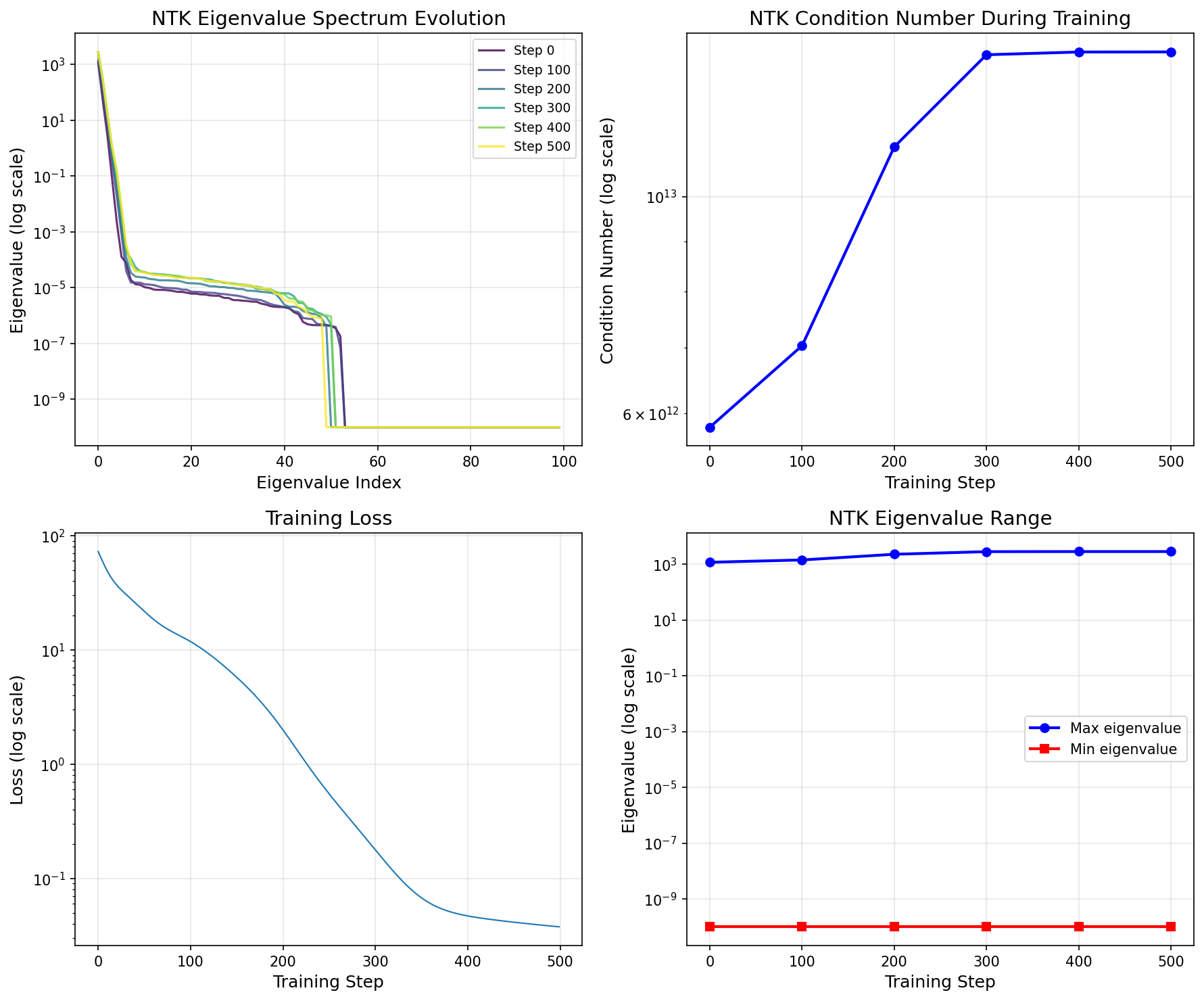
Key Result: NTK eigenvalue analysis reveals condition numbers of ~10^12, indicating significant spectral bias. Large eigenvalue gaps cause slow convergence for certain solution modes.
What You'll Learn
- Compute the empirical NTK matrix for a PINN model
- Analyze eigenvalue spectrum to understand training dynamics
- Detect spectral bias from eigenvalue distribution
- Track NTK evolution during training (finite-width effects)
- Predict convergence rates from NTK spectrum
Coming from Other Frameworks?
| Framework | NTK Support | Opifex Equivalent |
|---|---|---|
| DeepXDE | Not implemented | NTKWrapper.compute_ntk() |
| PhysicsNeMo | Not implemented | compute_eigenvalues() |
| NeuralOperator | Not implemented | detect_spectral_bias() |
Opifex is unique in providing built-in NTK analysis tools for PINNs.
Files
- Python script:
examples/advanced-training/ntk_analysis.py - Jupyter notebook:
examples/advanced-training/ntk_analysis.ipynb
Quick Start
Run the script
Run the notebook
Core Concepts
Neural Tangent Kernel Theory
The NTK Θ(x, x') captures how the network output at x changes when training on x':
For gradient descent training: - Large eigenvalues → fast convergence for those modes - Small eigenvalues → slow convergence (spectral bias) - Condition number → ratio of max to min eigenvalue
graph TD
    A[PINN Model] --> B[Compute Jacobian J]
    B --> C[NTK = J @ J.T]
    C --> D[Eigendecomposition]
    D --> E[Eigenvalues λ]
    D --> F[Eigenvectors v]
    E --> G[Condition Number]
    E --> H[Spectral Bias]
    E --> I[Convergence Rate]
Key Diagnostics
| Metric | Formula | Interpretation |
|---|---|---|
| Condition Number | λ_max / λ_min | Training difficulty |
| Effective Rank | (Σλ)² / Σλ² | Active learning modes |
| Spectral Bias | log(λ_max / λ_min) | Frequency learning gap |
Implementation
Step 1: Define PINN
class PoissonPINN(nnx.Module):
    """Simple PINN for 1D Poisson equation."""

    def __init__(self, hidden_dims: list[int] | None = None, *, rngs: nnx.Rngs):
        super().__init__()
        if hidden_dims is None:
            hidden_dims = [32, 32]
        # Build network layers...
Terminal Output:
Step 2: Compute Initial NTK
from opifex.core.physics.ntk.wrapper import NTKWrapper
from opifex.core.physics.ntk.diagnostics import detect_spectral_bias

# Create NTK wrapper
ntk_wrapper = NTKWrapper(pinn)

# Compute NTK matrix and eigenvalues
ntk_matrix = ntk_wrapper.compute_ntk(x_ntk)
eigenvalues = ntk_wrapper.compute_eigenvalues(x_ntk)
Terminal Output:
Computing initial NTK...
--------------------------------------------------
  NTK matrix shape: (100, 100)
  Eigenvalues range: [1.000000e-10, 1.162607e+03]

Initial NTK Diagnostics:
  Condition number: 5.81e+12
  Effective rank: 1.20
  Spectral bias indicator: 30.08
  Slow-converging modes: 97/100
Step 3: Track NTK During Training
for step in range(TRAINING_STEPS):
    loss = train_step(pinn, opt, x_train, x_bc)

    if step % NTK_COMPUTE_FREQUENCY == 0:
        eigenvalues = ntk_wrapper.compute_eigenvalues(x_ntk)
        cond = compute_condition_number(eigenvalues)
        print(f"Step {step}: loss={loss:.6e}, cond={cond:.2e}")
Terminal Output:
Training PINN with NTK tracking...
--------------------------------------------------
  Step    0: loss=7.256213e+01, cond=5.81e+12
  Step  100: loss=1.181392e+01, cond=7.04e+12
  Step  200: loss=1.993417e+00, cond=1.12e+13
  Step  300: loss=1.775255e-01, cond=1.40e+13
  Step  400: loss=4.693647e-02, cond=1.41e+13
  Step  500: loss=3.767164e-02, cond=1.41e+13
Visualization
NTK Eigenvalue Spectrum Evolution
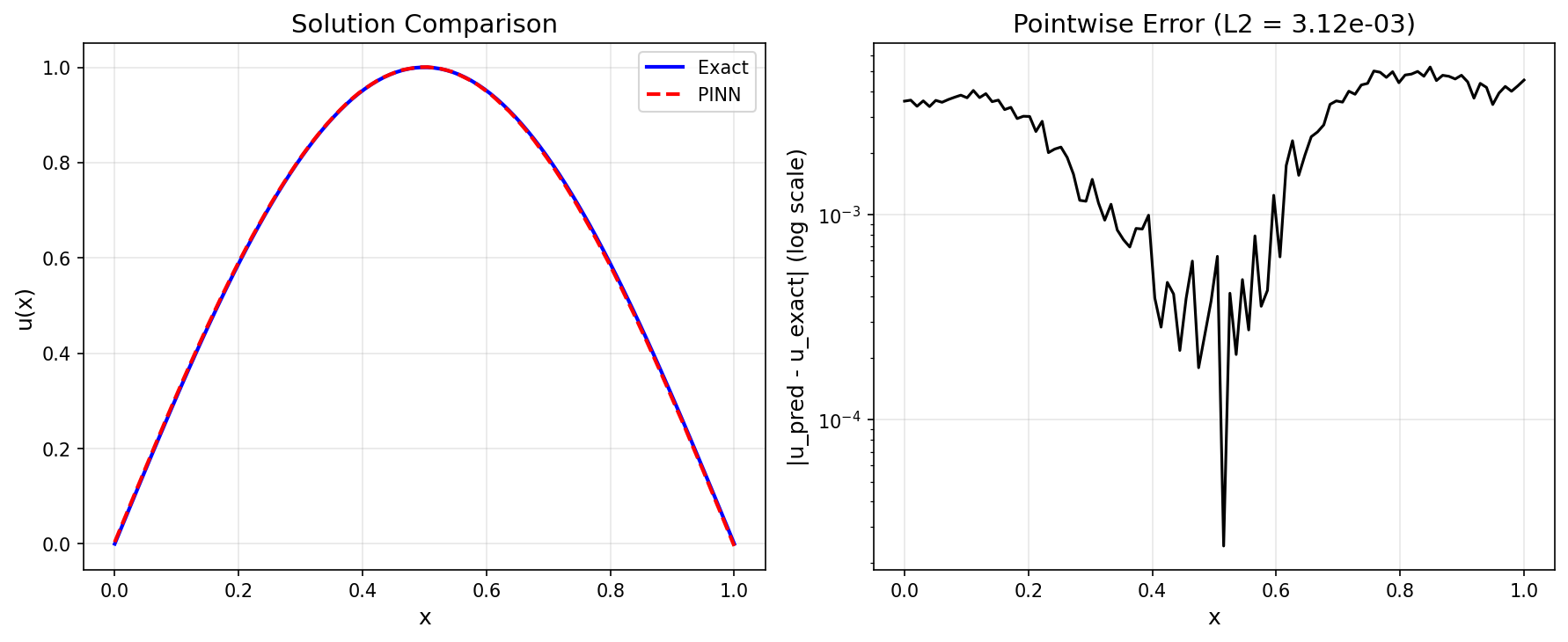
Solution Comparison
Results Summary
| Metric | Initial | Final |
|---|---|---|
| Condition Number | 5.81e+12 | 1.41e+13 |
| Effective Rank | 1.20 | 1.40 |
| Training Loss | 7.26e+01 | 3.77e-02 |
| L2 Error | - | 3.12e-03 |
Key Insights:
- High condition number indicates spectral bias
- NTK evolves during training (finite-width effect)
- Low effective rank means few modes are actively learned
- Understanding NTK helps diagnose PINN training difficulties
Next Steps
Experiments to Try
- Increase network width: How does it affect condition number?
- Different activations: Compare tanh vs ReLU vs GELU
- Learning rate tuning: Based on NTK eigenvalues
- Multi-scale problems: Analyze NTK for high-frequency solutions
Related Examples
- GradNorm Loss Balancing - Automatic multi-task balancing
- Adaptive Sampling - Residual-based point distribution
- Poisson PINN - Basic PINN training
API Reference
Troubleshooting
NTK computation is slow
- Reduce
N_COLLOCATIONfor NTK computation - Use a subset of domain points for diagnostics
- NTK computation scales as O(n² * p) where n=points, p=parameters
Negative eigenvalues
- Small negative eigenvalues are numerical noise
- Use
jnp.maximum(eigenvalues, 1e-10)to clip - Check if NTK matrix is symmetric (should be for same input points)
Very high condition number
- Expected for ill-conditioned problems
- Consider using spectral bias mitigation techniques
- Multi-scale input encoding can help