Poisson Equation PINN
| Metadata | Value |
|---|---|
| Level | Intermediate |
| Runtime | ~2 min (CPU) / ~30s (GPU) |
| Prerequisites | JAX, Flax NNX, calculus basics |
| Format | Python + Jupyter |
| Memory | ~500 MB RAM |
Overview
This tutorial demonstrates solving the 2D Poisson equation using a Physics-Informed Neural Network (PINN). The Poisson equation is fundamental to electrostatics, heat conduction, and potential flow theory.
Unlike data-driven neural operators (FNO, DeepONet), PINNs embed the governing PDE directly into the loss function, requiring no simulation data. The network learns to satisfy both the PDE residual and boundary conditions simultaneously.
What You'll Learn
- Implement a PINN architecture for elliptic PDEs
- Compute PDE residuals using JAX automatic differentiation (Hessian)
- Generate interior and boundary collocation points
- Balance physics loss and boundary loss with weighting
- Validate against known analytical solutions
Coming from DeepXDE?
If you are familiar with the DeepXDE library:
| DeepXDE | Opifex (JAX) |
|---|---|
dde.geometry.Rectangle([0,0], [1,1]) |
jax.random.uniform(key, (N, 2)) for interior |
dde.grad.hessian(y, x) |
jax.hessian(u_fn)(xy) + jnp.trace() |
dde.icbc.DirichletBC(geom, func, boundary) |
Manual boundary sampling + loss term |
dde.data.PDE(geom, pde, bc, num_domain, num_boundary) |
Explicit collocation arrays |
model.compile("adam", lr=1e-3) |
nnx.Optimizer(pinn, optax.adam(lr), wrt=nnx.Param) |
model.train(iterations=10000) |
Custom training loop with @nnx.jit |
Key differences:
- Pure JAX autodiff: Use
jax.hessiandirectly instead of custom gradient APIs - Explicit collocation: Collocation points are simple JAX arrays, not data objects
- Manual loss balancing: Explicit control over loss weights (
lambda_bc) - JIT compilation: Entire training step is XLA-compiled for GPU acceleration
Files
- Python Script:
examples/pinns/poisson.py - Jupyter Notebook:
examples/pinns/poisson.ipynb
Quick Start
Run the Python Script
Run the Jupyter Notebook
Core Concepts
PINN Architecture
PINNs solve PDEs by training a neural network to minimize physics residuals:
graph TB
    subgraph Input["Collocation Points"]
        A["Interior Points<br/>(x, y) in Ω"]
        B["Boundary Points<br/>(x, y) on ∂Ω"]
    end

    subgraph PINN["Neural Network u_θ(x, y)"]
        C["Linear + tanh<br/>64 units"]
        D["Linear + tanh<br/>64 units"]
        E["Linear + tanh<br/>64 units"]
        F["Linear<br/>1 unit"]
    end

    subgraph Loss["Physics-Informed Loss"]
        G["PDE Residual<br/>|-∇²u - f|²"]
        H["Boundary Loss<br/>|u(∂Ω)|²"]
        I["Total Loss<br/>L_pde + λ·L_bc"]
    end

    A --> C --> D --> E --> F --> G
    B --> C
    F --> H
    G --> I
    H --> I

    style G fill:#e3f2fd,stroke:#1976d2
    style H fill:#fff3e0,stroke:#f57c00
    style I fill:#c8e6c9,stroke:#388e3c
Poisson Equation
The Poisson equation is a fundamental elliptic PDE:
where \(\nabla^2 = \frac{\partial^2}{\partial x^2} + \frac{\partial^2}{\partial y^2}\) is the Laplacian.
| Component | This Example |
|---|---|
| Domain | \([0,1] \times [0,1]\) unit square |
| Source term | \(f(x,y) = 2\pi^2 \sin(\pi x) \sin(\pi y)\) |
| Boundary | Dirichlet: \(u = 0\) on \(\partial\Omega\) |
| Analytical solution | \(u(x,y) = \sin(\pi x) \sin(\pi y)\) |
Computing the Laplacian
The Laplacian is computed using JAX's Hessian and trace:
def compute_laplacian(pinn, xy):
    def u_scalar(xy_single):
        return pinn(xy_single.reshape(1, 2)).squeeze()

    def laplacian_single(xy_single):
        hessian = jax.hessian(u_scalar)(xy_single)
        return jnp.trace(hessian)  # ∇²u = tr(H)

    return jax.vmap(laplacian_single)(xy)
Implementation
Step 1: Imports and Setup
Terminal Output:
======================================================================
Opifex Example: Poisson Equation PINN
======================================================================
JAX backend: gpu
JAX devices: [CudaDevice(id=0)]
Interior points: 2000, Boundary points: 500
Epochs: 5000, Learning rate: 0.001
Network: [64, 64, 64]
Step 2: Define the Problem
def source_term(x, y):
    """Source term f(x, y) for the Poisson equation."""
    return 2.0 * jnp.pi**2 * jnp.sin(jnp.pi * x) * jnp.sin(jnp.pi * y)

def analytical_solution(x, y):
    """Analytical solution u(x, y)."""
    return jnp.sin(jnp.pi * x) * jnp.sin(jnp.pi * y)
Terminal Output:
Problem: -∇²u = f(x,y) on [0,1]²
Source term: f(x,y) = 2π² sin(πx) sin(πy)
Boundary: u = 0 (Dirichlet)
Analytical solution: u(x,y) = sin(πx) sin(πy)
Step 3: Create the PINN
class PoissonPINN(nnx.Module):
    def __init__(self, hidden_dims: list[int], *, rngs: nnx.Rngs):
        layers = []
        in_features = 2  # (x, y)
        for hidden_dim in hidden_dims:
            layers.append(nnx.Linear(in_features, hidden_dim, rngs=rngs))
            in_features = hidden_dim
        layers.append(nnx.Linear(in_features, 1, rngs=rngs))
        self.layers = nnx.List(layers)

    def __call__(self, xy: jax.Array) -> jax.Array:
        h = xy
        for layer in self.layers[:-1]:
            h = jnp.tanh(layer(h))
        return self.layers[-1](h)

pinn = PoissonPINN(hidden_dims=[64, 64, 64], rngs=nnx.Rngs(42))
Terminal Output:
Step 4: Generate Collocation Points
# Interior points
x_interior = jax.random.uniform(key, (N_INTERIOR, 2))

# Boundary points (sample all 4 edges)
bottom = jnp.column_stack([jax.random.uniform(key, (n,)), jnp.zeros(n)])
top = jnp.column_stack([jax.random.uniform(key, (n,)), jnp.ones(n)])
left = jnp.column_stack([jnp.zeros(n), jax.random.uniform(key, (n,))])
right = jnp.column_stack([jnp.ones(n), jax.random.uniform(key, (n,))])
x_boundary = jnp.concatenate([bottom, top, left, right], axis=0)
Terminal Output:
Step 5: Define Physics-Informed Loss
def total_loss(pinn, x_int, x_bc, lambda_bc=10.0):
    loss_pde = pde_residual_loss(pinn, x_int)
    loss_bc = boundary_loss(pinn, x_bc)
    return loss_pde + lambda_bc * loss_bc
Step 6: Training
Terminal Output:
Training PINN...
  Epoch     1/5000: loss=9.788428e+01
  Epoch  1000/5000: loss=5.333988e-02
  Epoch  2000/5000: loss=6.953341e-03
  Epoch  3000/5000: loss=3.755849e-03
  Epoch  4000/5000: loss=4.713943e-03
  Epoch  5000/5000: loss=6.020937e-04
Final loss: 6.020937e-04
Step 7: Evaluation
Terminal Output:
Evaluating PINN...
Relative L2 error:   4.711105e-03
Maximum point error: 2.005570e-02
Mean point error:    1.674831e-03
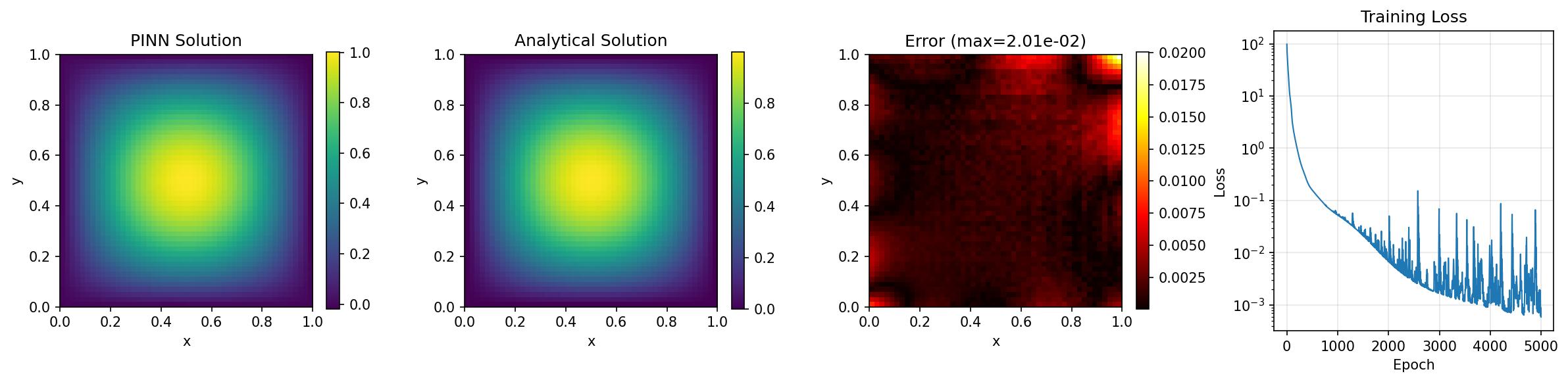
Visualization
Solution Comparison
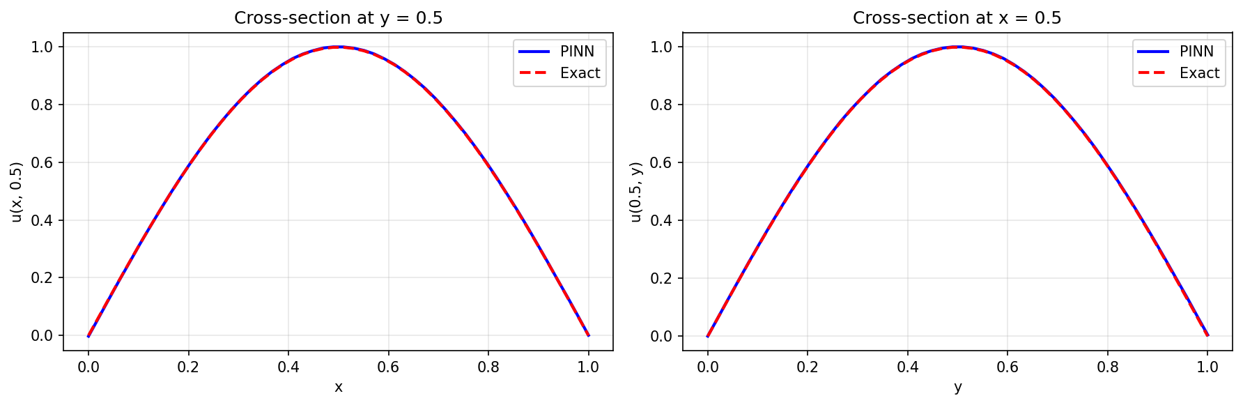
Cross-Sections
Results Summary
| Metric | Value |
|---|---|
| Final Loss | 6.02e-04 |
| Relative L2 Error | 0.47% |
| Maximum Point Error | 2.01e-02 |
| Mean Point Error | 1.67e-03 |
| Parameters | 8,577 |
| Training Epochs | 5,000 |
Next Steps
Experiments to Try
- Increase epochs: Train for 10,000+ epochs to reduce error below 0.1%
- Larger network: Try
hidden_dims=[128, 128, 128, 128]for higher accuracy - More collocation points: Use 10,000 interior points for better coverage
- Adaptive sampling: Concentrate points where error is high (residual-based)
- Different BCs: Try Neumann or mixed boundary conditions
Related Examples
| Example | Level | What You'll Learn |
|---|---|---|
| Heat Equation PINN | Intermediate | Time-dependent PDEs |
| FNO on Darcy Flow | Intermediate | Data-driven alternative |
| Domain Decomposition | Advanced | Large domain problems |
API Reference
nnx.Linear- Linear layernnx.Optimizer- Optimizer wrapperjax.hessian- Hessian computationjax.vmap- Vectorized mapping
Troubleshooting
Loss not decreasing
Symptom: Training loss stays flat or decreases very slowly.
Cause: Learning rate too low, or boundary loss weight too high/low.
Solution: Adjust learning rate and boundary weight:
# Try higher learning rate initially
LEARNING_RATE = 1e-2  # Then decay

# Adjust boundary weight
lambda_bc = 1.0  # Lower if boundary dominates
lambda_bc = 100.0  # Higher if solution doesn't satisfy BCs
PINN predicts constant zero
Symptom: All predictions are approximately zero.
Cause: Boundary loss dominates (trivial solution satisfies u=0 everywhere).
Solution: The source term f(x,y) must create a non-trivial solution. Verify:
# Check source term is non-zero
f_values = source_term(x_interior[:, 0], x_interior[:, 1])
print(f"Source term range: [{f_values.min()}, {f_values.max()}]")
Slow convergence
Symptom: Need many epochs (>100,000) to converge.
Cause: Network architecture not suited for the solution smoothness.
Solution: Use tanh activation (smooth) for smooth solutions, increase network depth:
# Deeper network for complex solutions
hidden_dims = [64, 64, 64, 64]

# Use tanh for smooth PDEs
h = jnp.tanh(layer(h))  # Not ReLU
Memory error with many collocation points
Symptom: OOM error when increasing N_INTERIOR.
Cause: Computing Hessian for all points simultaneously.
Solution: Use mini-batching in the training loop: