Training a Neural Exchange-Correlation Functional¶

Metadata	Value
Level	Advanced
Runtime	~15 sec (GPU) / ~2 min (CPU)
Prerequisites	JAX, Flax NNX, DFT Basics
Format	Python + Jupyter
Memory	~1 GB RAM

Overview¶

This example demonstrates training a neural exchange-correlation (XC) functional from electron density data. The neural XC functional learns to predict exchange-correlation energies from electron density, going beyond traditional LDA/GGA approximations.

Key Concepts:

Exchange-Correlation Energy: The challenging part of DFT
Density Feature Extraction: Physics-informed input processing
Attention Mechanism: Captures non-local electron correlations
Physics Constraints: Ensures negative XC energy and proper scaling

What You'll Learn¶

Generate synthetic training data with LDA reference energies
Configure NeuralXCFunctional with attention and advanced features
Train using MSE loss to match reference XC energies
Evaluate accuracy with R² and correlation metrics
Verify physics constraints (negative XC energy)

Coming from PyTorch/DeepChem?¶

Traditional ML (PyTorch)	Opifex Neural XC
Generic MLP	Physics-informed architecture
Standard features	Density + gradients + kinetic energy
No physics constraints	Built-in negativity + scaling constraints
`torch.nn.Module`	`NeuralXCFunctional`
`model(x)`	`model(density, gradients)`

Key differences:

Physics-aware: Features include reduced gradient, Fermi wavevector
Attention for non-locality: Captures beyond-local correlations
Constrained output: Guarantees physically valid XC energy
JAX-native: Automatic differentiation for functional derivatives

Files¶

Python Script: examples/quantum-chemistry/neural_xc_functional.py
Jupyter Notebook: examples/quantum-chemistry/neural_xc_functional.ipynb

Quick Start¶

Run the Python Script¶

source activate.sh && python examples/quantum-chemistry/neural_xc_functional.py

Run the Jupyter Notebook¶

jupyter lab examples/quantum-chemistry/neural_xc_functional.ipynb

Core Concepts¶

Exchange-Correlation Energy¶

In DFT, the XC energy captures: - Exchange: Pauli exclusion effects - Correlation: Electron-electron interactions beyond mean-field

The LDA approximation: $$E_{xc}^{LDA} = -C_x \\int \\rho^{4/3} dr$$

Neural XC functionals can learn more accurate energy predictions by: - Including gradient information (GGA-like) - Using attention for non-local correlations - Learning from high-level ab initio data

Neural XC Architecture¶

Density ρ(r) ──┐
               ├─→ Feature Extractor ─→ Attention ─→ MLP ─→ E_xc(r)
Gradients ∇ρ ──┘

Feature Extractor computes: - Log density: log(ρ) - Gradient magnitude: |∇ρ| - Reduced gradient: |∇ρ| / ρ^(4/3) - Kinetic energy density - Fermi wavevector

Physics Constraints¶

The neural XC functional enforces: 1. Negative energy: XC energy should be attractive 2. Density scaling: Proper behavior at low densities 3. Numerical stability: Clipping and smoothing

Implementation¶

Step 1: Generate Training Data¶

def compute_lda_xc_energy(density):
    """Compute LDA exchange-correlation energy."""
    c_x = 0.738  # Exchange coefficient
    exchange = -c_x * jnp.power(density, 4/3)

    c_c = 0.044  # Correlation coefficient
    correlation = -c_c * density * jnp.log1p(density)

    return exchange + correlation

# Generate synthetic densities
train_densities = jnp.stack([
    generate_density_sample(key, grid_points)
    for key in train_keys
])
train_xc_ref = jnp.stack([
    compute_lda_xc_energy(d) for d in train_densities
])

Terminal Output:

Generating training data...
--------------------------------------------------
  Training samples: 500
  Test samples: 100
  Grid points per sample: 32

  Train densities shape: (500, 32)
  Train gradients shape: (500, 32, 3)
  Train XC reference shape: (500, 32)

Step 2: Create Neural XC Functional¶

from opifex.neural.quantum import NeuralXCFunctional
from flax import nnx

model = NeuralXCFunctional(
    hidden_sizes=(64, 64, 32),
    activation=nnx.gelu,
    use_attention=True,
    num_attention_heads=4,
    use_advanced_features=True,
    dropout_rate=0.0,
    rngs=nnx.Rngs(42),
)

Terminal Output:

Creating Neural XC Functional...
--------------------------------------------------
  Hidden sizes: (64, 64, 32)
  Use attention: True
  Attention heads: 4
  Use advanced features: True
  Total parameters: 23,303

Step 3: Train the Model¶

def loss_fn(model, densities, gradients, targets):
    predictions = model(densities, gradients, deterministic=True)
    return jnp.mean((predictions - targets) ** 2)

optimizer = nnx.Optimizer(model, optax.adam(1e-3), wrt=nnx.Param)

@nnx.jit
def train_step(model, optimizer, densities, gradients, targets):
    loss, grads = nnx.value_and_grad(loss_fn)(model, densities, gradients, targets)
    optimizer.update(model, grads)
    return loss

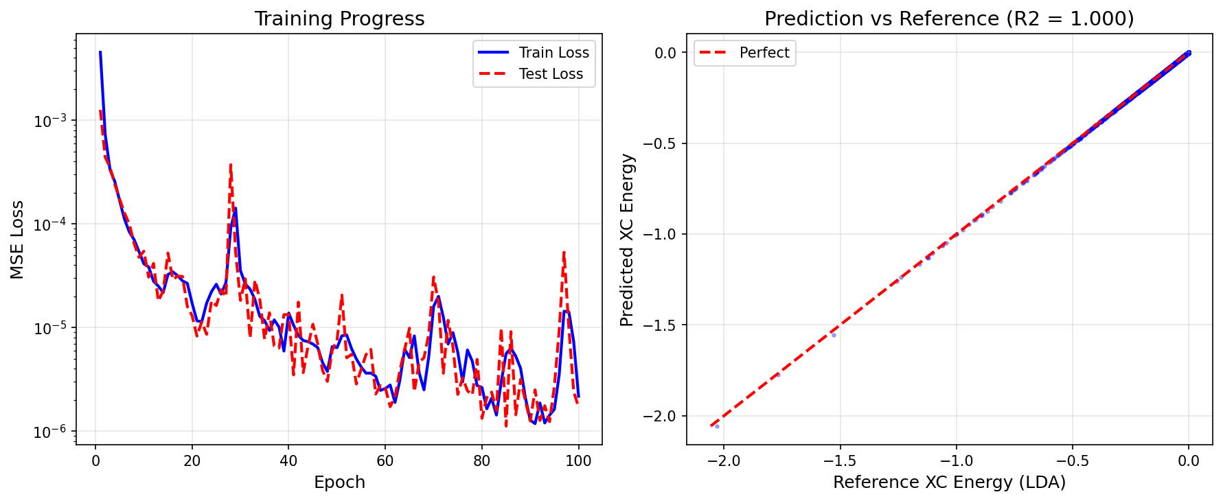
Terminal Output:

Training Neural XC Functional...
--------------------------------------------------
  Epoch   1/100: train_loss = 0.004533, test_loss = 0.001263
  Epoch  10/100: train_loss = 0.000041, test_loss = 0.000054
  Epoch  20/100: train_loss = 0.000017, test_loss = 0.000013
  Epoch  50/100: train_loss = 0.000006, test_loss = 0.000008
  Epoch 100/100: train_loss = 0.000002, test_loss = 0.000002

Training complete!
  Training time: 10.3s
  Final train loss: 0.000002
  Final test loss: 0.000002

Step 4: Evaluate Performance¶

test_predictions = model(test_densities, test_gradients, deterministic=True)

mse = jnp.mean((test_predictions - test_xc_ref) ** 2)
r2 = 1 - jnp.sum((test_xc_ref - test_predictions) ** 2) / \
         jnp.sum((test_xc_ref - jnp.mean(test_xc_ref)) ** 2)

Terminal Output:

Evaluating model performance...
--------------------------------------------------
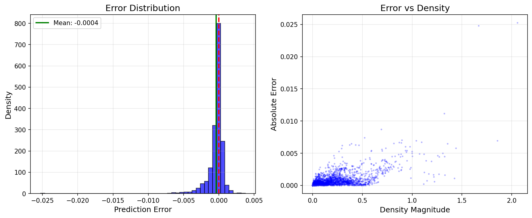
  Mean Squared Error (MSE): 1.703340e-06
  Mean Absolute Error (MAE): 6.605385e-04
  R-squared (R2): 0.9999
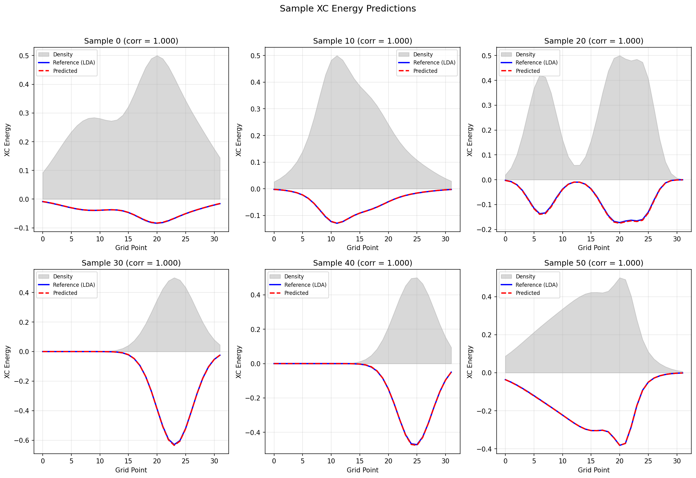
  Mean Correlation: 1.0000

Physics Constraint Verification:
  XC energy negative: 100.0% of predictions

Visualization¶

Training Curves

Sample Predictions

Error Analysis

Results Summary¶

Metric	Value
Hidden sizes	(64, 64, 32)
Attention heads	4
Parameters	23,303
Training samples	500
Training time	~10s
Final MSE	1.70e-6
R-squared	0.9999
Mean correlation	1.0000
Negative XC energy	100%

Next Steps¶

Experiments to Try¶

More hidden layers: Try (128, 128, 64, 32) for complex patterns
More attention heads: 8 heads may capture finer correlations
Disable attention: Compare with/without for local vs non-local effects
Real DFT data: Train on reference data from PySCF or Gaussian

Example	Level	What You'll Learn
Neural DFT	Advanced	Full DFT energy calculation
FNO on Darcy	Beginner	Data-driven operator learning

API Reference¶

NeuralXCFunctional: Main neural XC functional class
DensityFeatureExtractor: Physics-informed feature extraction
MultiHeadAttention: Attention for non-local correlations
compute_functional_derivative(): Compute XC potential V_xc
assess_chemical_accuracy(): Built-in accuracy assessment

Troubleshooting¶

Issue	Solution
NaN in training	Reduce learning rate, check density range
Poor R²	More training data, larger model
Positive XC energy	Check physics constraints are enabled
Slow training	Use GPU, reduce batch size

Advanced Usage¶

Computing the XC Potential:

# Functional derivative for Kohn-Sham equations
xc_potential = model.compute_functional_derivative(
    density, gradients, deterministic=True
)

Using with Neural DFT:

from opifex.neural.quantum import NeuralDFT

# The neural DFT framework uses NeuralXCFunctional internally
neural_dft = NeuralDFT(
    xc_functional_type="neural",  # Uses NeuralXCFunctional
    rngs=rngs,
)

Training a Neural Exchange-Correlation Functional¶

Overview¶

What You'll Learn¶

Coming from PyTorch/DeepChem?¶

Files¶

Quick Start¶

Run the Python Script¶

Run the Jupyter Notebook¶

Core Concepts¶

Exchange-Correlation Energy¶

Neural XC Architecture¶

Physics Constraints¶

Implementation¶

Step 1: Generate Training Data¶

Step 2: Create Neural XC Functional¶

Step 3: Train the Model¶

Step 4: Evaluate Performance¶

Visualization¶

Results Summary¶

Next Steps¶

Experiments to Try¶

Related Examples¶

API Reference¶

Troubleshooting¶

Advanced Usage¶