Local FNO on Darcy Flow

Metadata	Value
Level	Intermediate
Runtime	~3 min (CPU) / ~30s (GPU)
Prerequisites	JAX, Flax NNX, FNO basics
Format	Python + Jupyter
Memory	~1 GB RAM

Overview

This tutorial demonstrates training a Local Fourier Neural Operator (LocalFNO) on the Darcy flow problem. LocalFNO combines global spectral convolutions with local spatial convolutions to capture both long-range dependencies and fine-grained local features.

The key insight is that many physical systems exhibit both global patterns (e.g., overall flow direction) and local features (e.g., boundary layers, sharp gradients). LocalFNO addresses this by processing inputs through both spectral (global) and convolutional (local) branches, then combining the results.

What You'll Learn

1. Understand LocalFNO architecture: spectral + local convolution branches
2. Create a LocalFourierNeuralOperator with configurable kernel size
3. Compare LocalFNO vs standard FNO on the same problem
4. Analyze the trade-off between accuracy and parameter count

Coming from NeuralOperator (PyTorch)?

If you are familiar with the neuraloperator library:

NeuralOperator (PyTorch)	Opifex (JAX)
No built-in LocalFNO	LocalFourierNeuralOperator(..., kernel_size=3)
Manual local convolution layers	Built-in spectral + local branch combination
torch.compile	@nnx.jit for XLA compilation
torch.nn.Conv2d for local ops	nnx.Conv with automatic NHWC/NCHW conversion

Key differences:

1. Integrated local branch: Opifex's LocalFNO has built-in local convolution per layer
2. Mixing weight: Configurable mixing_weight controls spectral vs local balance
3. Residual connections: Optional skip connections for improved gradient flow
4. Factory functions: create_turbulence_local_fno(), create_wave_local_fno() presets

Files

• Python Script: examples/neural-operators/local_fno_darcy.py
• Jupyter Notebook: examples/neural-operators/local_fno_darcy.ipynb

Quick Start

Run the Python Script

source activate.sh && python examples/neural-operators/local_fno_darcy.py

Run the Jupyter Notebook

jupyter lab examples/neural-operators/local_fno_darcy.ipynb

Core Concepts

LocalFNO Architecture

LocalFNO extends FNO by adding a local convolution branch in each layer:

graph LR
    subgraph Input
        A["Permeability Field<br/>a(x) : (1, 32, 32)"]
    end

    subgraph LocalFNO["Local Fourier Neural Operator"]
        B["Lifting<br/>1 → 32 channels"]
        C["LocalFourierLayer 1"]
        D["LocalFourierLayer 2"]
        E["LocalFourierLayer 3"]
        F["LocalFourierLayer 4"]
        G["Projection<br/>32 → 1 channels"]
    end

    subgraph Output
        H["Pressure Field<br/>u(x) : (1, 32, 32)"]
    end

    A --> B --> C --> D --> E --> F --> G --> H

LocalFourierLayer Detail

Each layer processes input through two parallel branches:

graph TB
    A["Input x"] --> B["Spectral Branch<br/>(FFT → Spectral Conv → iFFT)"]
    A --> C["Local Branch<br/>(Conv2D, kernel=3)"]
    B --> D["α × spectral"]
    C --> E["(1-α) × local"]
    D --> F["Sum + Skip"]
    E --> F
    A --> F
    F --> G["GELU Activation"]
    G --> H["Output"]

    style B fill:#e3f2fd,stroke:#1976d2
    style C fill:#fff3e0,stroke:#f57c00

Where α is the mixing_weight parameter (default 0.5).

When to Use LocalFNO

Problem Type	Standard FNO	LocalFNO
Smooth solutions	Good	Comparable
Sharp gradients	Limited	Better
Boundary layers	Limited	Better
Turbulence (multi-scale)	Good	Better
Memory-constrained	Better	More params

Implementation

Step 1: Imports and Setup

import jax
from flax import nnx

from opifex.data.loaders import create_darcy_loader
from opifex.neural.operators.fno.local import LocalFourierNeuralOperator
from opifex.neural.operators.fno.base import FourierNeuralOperator

Terminal Output:

======================================================================
Opifex Example: Local FNO on Darcy Flow
======================================================================
JAX backend: gpu
JAX devices: [CudaDevice(id=0)]
Resolution: 32x32
Training samples: 200, Test samples: 50
Batch size: 16, Epochs: 20
FNO config: modes=(12, 12), width=32, layers=4
Local kernel size: 3

Step 2: Data Loading

train_loader = create_darcy_loader(
    n_samples=200,
    batch_size=16,
    resolution=32,
    shuffle=True,
    seed=42,
)

Terminal Output:

Generating Darcy flow data...
Training data: X=(16, 1, 32, 32), Y=(16, 1, 32, 32)
Test data:     X=(50, 1, 32, 32), Y=(50, 1, 32, 32)

Step 3: Model Creation

local_fno = LocalFourierNeuralOperator(
    in_channels=1,
    out_channels=1,
    hidden_channels=32,
    modes=(12, 12),
    num_layers=4,
    kernel_size=3,
    use_residual_connections=True,
    rngs=nnx.Rngs(42),
)

Terminal Output:

Creating LocalFNO model...
LocalFNO parameters: 365,035

Creating standard FNO for comparison...
Standard FNO parameters: 53,473
LocalFNO overhead: 582.7%

Step 4: Training

opt = nnx.Optimizer(model, optax.adam(1e-3), wrt=nnx.Param)

@nnx.jit
def train_step(model, opt, x, y):
    def loss_fn(model):
        y_pred = model(x)
        return jnp.mean((y_pred - y) ** 2)

    loss, grads = nnx.value_and_grad(loss_fn)(model)
    opt.update(model, grads)
    return loss

Terminal Output:

Training LocalFNO...
  Epoch   1/20: loss=0.518433
  Epoch   5/20: loss=0.021340
  Epoch  10/20: loss=0.005847
  Epoch  15/20: loss=0.008613
  Epoch  20/20: loss=0.001378
Final LocalFNO loss: 1.377639e-03

Training Standard FNO...
  Epoch   1/20: loss=0.045024
  Epoch   5/20: loss=0.013370
  Epoch  10/20: loss=0.000658
  Epoch  15/20: loss=0.002363
  Epoch  20/20: loss=0.000476
Final FNO loss: 4.763597e-04

Step 5: Evaluation

Terminal Output:

Running evaluation...
LocalFNO Results:
  Test MSE:         0.000669
  Relative L2:      2.710133 (min=2.208369, max=4.282701)

Standard FNO Results:
  Test MSE:         0.000765
  Relative L2:      2.816077 (min=1.666520, max=4.716997)

Comparison:
  MSE improvement (LocalFNO vs FNO): +12.5%
  Rel L2 improvement: +3.8%

Visualization

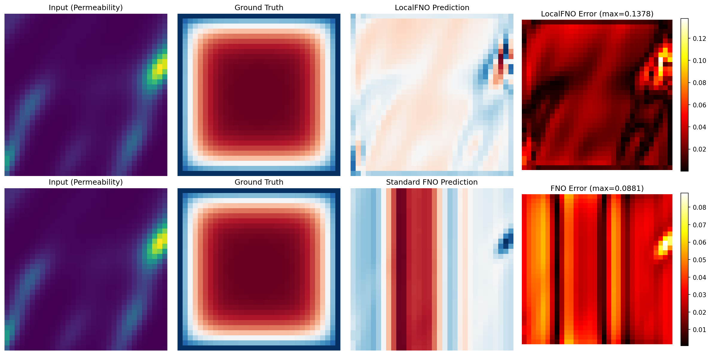
Predictions Comparison

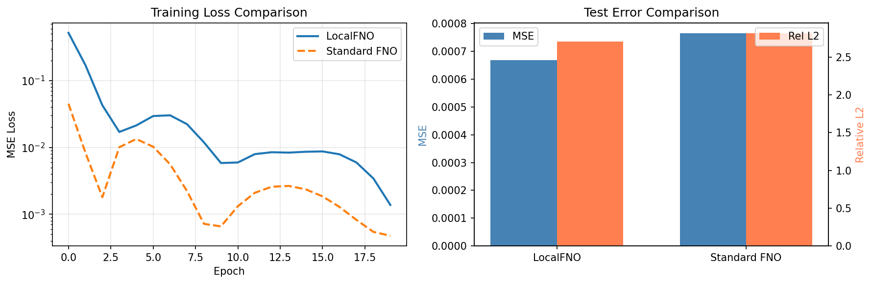
Training and Error Analysis

Results Summary

Metric	LocalFNO	Standard FNO
Test MSE	0.000669	0.000765
Relative L2 Error	2.71	2.82
Parameters	365,035	53,473
MSE Improvement	+12.5%	(baseline)

Next Steps

Experiments to Try

1. Vary kernel size: Try kernel_size=5 or kernel_size=7 for larger receptive fields
2. Adjust mixing weight: Use mixing_weight=0.3 to emphasize local features
3. Disable residual connections: Set use_residual_connections=False for comparison
4. Apply to turbulence: Use create_turbulence_local_fno() preset for turbulent flows

Related Examples

Example	Level	What You'll Learn
FNO on Darcy Flow	Intermediate	Standard FNO baseline
FNO on Burgers Equation	Intermediate	1D temporal evolution
U-FNO on Turbulence	Advanced	Multi-scale U-Net + FNO

API Reference

• LocalFourierNeuralOperator - Local FNO model class
• LocalFourierLayer - Individual local Fourier layer
• create_turbulence_local_fno - Preset for turbulent flows
• create_darcy_loader - Darcy flow data loader

Troubleshooting

LocalFNO uses more memory than expected

Symptom: RESOURCE_EXHAUSTED error or high memory usage.

Cause: LocalFNO has ~7x more parameters than standard FNO due to local convolution layers.

Solution: Reduce hidden channels or use smaller kernel size:

model = LocalFourierNeuralOperator(
    hidden_channels=16,  # Reduce from 32
    kernel_size=3,       # Keep small
    ...
)

Training is slower than standard FNO

Symptom: Each epoch takes significantly longer.

Cause: Additional local convolution operations add computational overhead.

Solution: LocalFNO is designed for problems where local features matter. For smooth problems, use standard FNO. For multi-scale problems, the accuracy improvement may justify the extra cost.

Relative L2 error is high

Symptom: Relative L2 > 1.0 despite low MSE.

Cause: The target field has small absolute values, making relative error high.

Solution: This is expected for some problems. Focus on MSE or increase training data:

train_loader = create_darcy_loader(n_samples=500, ...)  # More data