Allen-Cahn Equation PINN¶

Metadata	Value
Level	Advanced
Runtime	~5 min (GPU) / ~20 min (CPU)
Prerequisites	JAX, Flax NNX, reaction-diffusion
Format	Python + Jupyter
Memory	~1 GB RAM

Overview¶

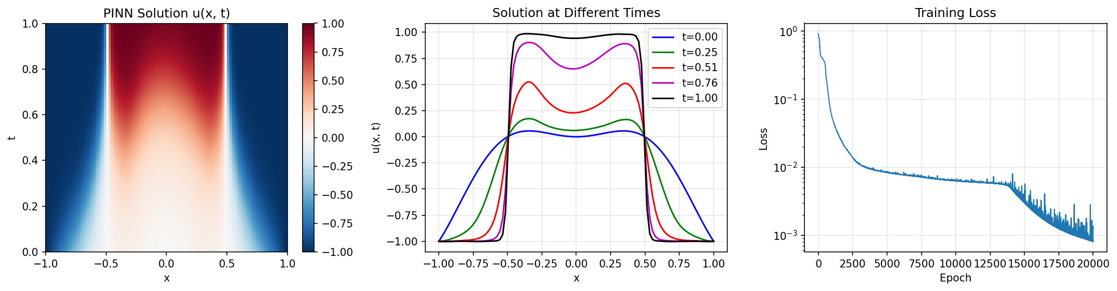
This tutorial demonstrates solving the Allen-Cahn equation using a Physics-Informed Neural Network (PINN). The Allen-Cahn equation is a reaction-diffusion PDE that models phase separation and interface dynamics in materials science, including solidification and crystal growth.

The equation features bistable dynamics with equilibria at \(u = \pm 1\), making it an excellent test for PINNs' ability to capture sharp transitions and nonlinear reaction terms.

What You'll Learn¶

Implement a PINN for reaction-diffusion PDEs with nonlinear terms
Apply hard constraints for both initial and boundary conditions
Handle bistable dynamics and phase transitions
Understand the balance between diffusion and reaction in PDEs
Visualize phase evolution over time

Coming from DeepXDE?¶

DeepXDE	Opifex (JAX)
`dde.geometry.GeometryXTime(geom, time)`	`jnp.column_stack([x, t])` for (x, t)
`net.apply_output_transform(transform)`	Hard constraint in `__call__` method
`5 * (y - y**3)` reaction term	`5.0 * (u - u**3)` in residual
`model.train(iterations=40000)`	20000 epochs (faster demo)

Key differences:

Hard constraint formula: u = x^2*cos(pi*x) + t*(1-x^2)*u_hat
Reduced epochs: 20000 vs 40000 (no L-BFGS refinement)
No external data: DeepXDE version loads .mat file for comparison

Files¶

Python Script: examples/pinns/allen_cahn.py
Jupyter Notebook: examples/pinns/allen_cahn.ipynb

Quick Start¶

Run the Python Script¶

source activate.sh && python examples/pinns/allen_cahn.py

Run the Jupyter Notebook¶

jupyter lab examples/pinns/allen_cahn.ipynb

Core Concepts¶

Allen-Cahn Equation¶

The Allen-Cahn equation is a reaction-diffusion PDE:

\[\frac{\partial u}{\partial t} = D \frac{\partial^2 u}{\partial x^2} + 5(u - u^3)\]

Component	This Example
Domain	\(x \in [-1, 1]\), \(t \in [0, 1]\)
Diffusion	\(D = 0.001\)
Reaction	\(5(u - u^3)\) with equilibria at \(u = -1, 0, +1\)
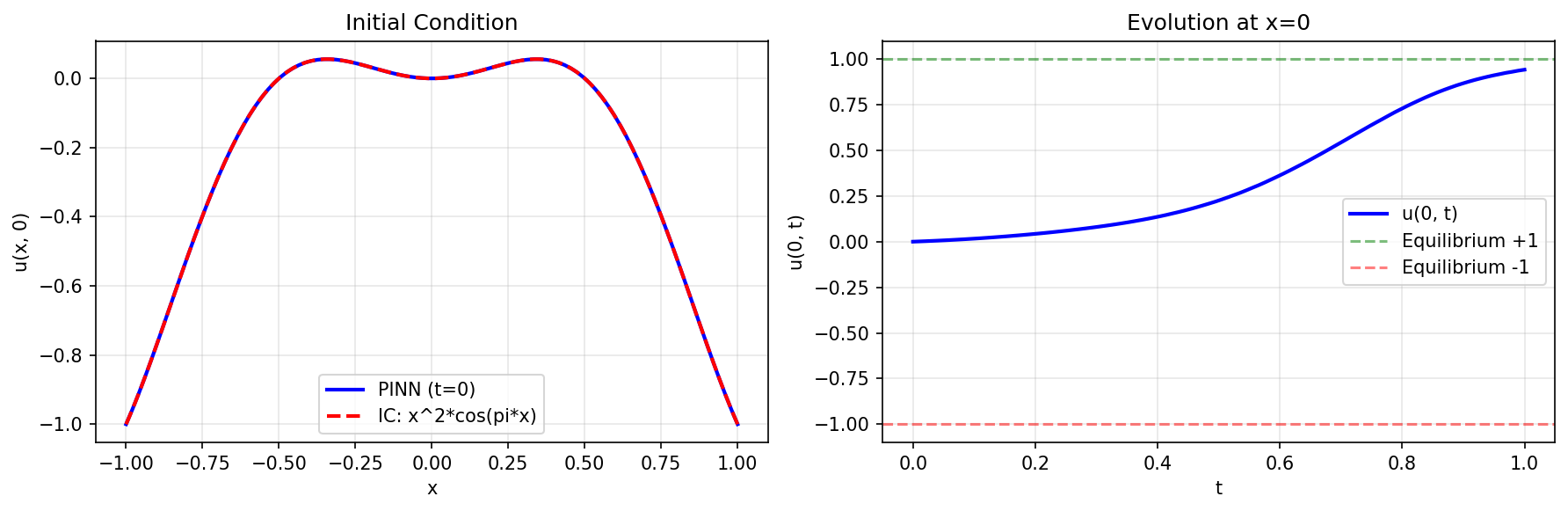
IC	\(u(x, 0) = x^2 \cos(\pi x)\)
BC	\(u(\pm 1, t) = -1\)

Physical Interpretation¶

Diffusion: Smooths spatial gradients (\(D \cdot u_{xx}\))
Reaction: Drives toward stable states \(u = \pm 1\)
Competition: Sharp interfaces form where phases meet
Bistability: \(u = 0\) is an unstable equilibrium; \(u = \pm 1\) are stable

Implementation¶

Step 1: Imports and Configuration¶

import jax
import jax.numpy as jnp
import optax
from flax import nnx

Terminal Output:

======================================================================
Opifex Example: Allen-Cahn Equation PINN
======================================================================
JAX backend: gpu
JAX devices: [CudaDevice(id=0)]
Diffusion coefficient: D = 0.001
Domain: x in [-1.0, 1.0], t in [0.0, 1.0]
Collocation: 8000 domain, 400 boundary, 800 initial
Network: [2] + [20, 20, 20] + [1]
Training: 20000 epochs @ lr=0.001

Step 2: Define the Problem¶

D = 0.001  # Diffusion coefficient

def initial_condition(x):
    """Initial condition: u(x, 0) = x^2 * cos(pi*x)."""
    return x**2 * jnp.cos(jnp.pi * x)

def boundary_value():
    """Boundary condition: u(+-1, t) = -1."""
    return -1.0

Terminal Output:

Allen-Cahn equation: du/dt = D*d2u/dx2 + 5*(u - u^3)
  Diffusion: D = 0.001
  Reaction: 5*(u - u^3) with equilibria at u = -1, 0, +1
  IC: u(x, 0) = x^2 * cos(pi*x)
  BC: u(-1, t) = u(1, t) = -1

Step 3: Create PINN with Hard Constraint¶

class AllenCahnPINN(nnx.Module):
    def __init__(self, hidden_dims: list[int], *, rngs: nnx.Rngs):
        super().__init__()
        layers = []
        in_features = 2  # (x, t)

        for hidden_dim in hidden_dims:
            layers.append(nnx.Linear(in_features, hidden_dim, rngs=rngs))
            in_features = hidden_dim

        layers.append(nnx.Linear(in_features, 1, rngs=rngs))
        self.layers = nnx.List(layers)

    def __call__(self, xt: jax.Array) -> jax.Array:
        """Forward pass with hard constraint."""
        # Neural network output
        h = xt
        for layer in self.layers[:-1]:
            h = jnp.tanh(layer(h))
        u_hat = self.layers[-1](h)

        # Hard constraint: u = x^2*cos(pi*x) + t*(1-x^2)*u_hat
        x, t = xt[:, 0:1], xt[:, 1:2]
        ic_term = x**2 * jnp.cos(jnp.pi * x)
        bc_mask = t * (1 - x**2)
        return ic_term + bc_mask * u_hat

pinn = AllenCahnPINN(hidden_dims=[20, 20, 20], rngs=nnx.Rngs(42))

This enforces:

At \(t=0\): \(u = x^2 \cos(\pi x)\) (IC)
At \(x=\pm 1\): \(u = \cos(\pm\pi) = -1\) (BC)

Terminal Output:

Creating PINN model...
PINN parameters: 921

Step 4: Generate Collocation Points¶

key = jax.random.PRNGKey(42)
keys = jax.random.split(key, 5)

# Domain interior points
x_domain = jax.random.uniform(keys[0], (N_DOMAIN,), minval=X_MIN, maxval=X_MAX)
t_domain = jax.random.uniform(keys[1], (N_DOMAIN,), minval=T_MIN, maxval=T_MAX)
xt_domain = jnp.column_stack([x_domain, t_domain])

Terminal Output:

Generating collocation points...
Domain points:   (8000, 2)
Boundary points: (400, 2)
Initial points:  (800, 2)

Step 5: Define Physics-Informed Loss¶

def compute_pde_residual(pinn, xt):
    """Compute Allen-Cahn PDE residual."""

    def u_scalar(xt_single):
        return pinn(xt_single.reshape(1, 2)).squeeze()

    def residual_single(xt_single):
        u = u_scalar(xt_single)
        grad_u = jax.grad(u_scalar)(xt_single)
        u_t = grad_u[1]

        def du_dx(xt_s):
            return jax.grad(u_scalar)(xt_s)[0]
        u_xx = jax.grad(du_dx)(xt_single)[0]

        # Allen-Cahn: u_t = D*u_xx + 5*(u - u^3)
        return u_t - D * u_xx - 5.0 * (u - u**3)

    return jax.vmap(residual_single)(xt)

def total_loss(pinn, xt_dom):
    """Total loss (PDE only with hard constraints)."""
    return pde_loss(pinn, xt_dom)

Step 6: Training¶

opt = nnx.Optimizer(pinn, optax.adam(LEARNING_RATE), wrt=nnx.Param)

@nnx.jit
def train_step(pinn, opt, xt_dom):
    def loss_fn(model):
        return total_loss(model, xt_dom)

    loss, grads = nnx.value_and_grad(loss_fn)(pinn)
    opt.update(pinn, grads)
    return loss

for epoch in range(EPOCHS):
    loss = train_step(pinn, opt, xt_domain)

Terminal Output:

Training PINN...
  Epoch     1/20000: loss=9.219739e-01
  Epoch  4000/20000: loss=9.446610e-03
  Epoch  8000/20000: loss=6.976590e-03
  Epoch 12000/20000: loss=5.941100e-03
  Epoch 16000/20000: loss=1.965126e-03
  Epoch 20000/20000: loss=1.216745e-03
Final loss: 1.216745e-03

Step 7: Evaluation¶

Terminal Output:

Evaluating PINN...
IC error (should be ~0):  0.000000e+00
BC error (should be ~0):  0.000000e+00
Mean PDE residual:        2.379521e-02

Visualization¶

Allen-Cahn Solution

Analysis

Results Summary¶

Metric	Value
Final Loss	1.22e-03
IC Error	0.0
BC Error	0.0
Mean PDE Residual	2.38e-02
Parameters	921
Training Epochs	20,000

Next Steps¶

Experiments to Try¶

More epochs: Train for 40000+ epochs to reduce residual
Add L-BFGS: Use second-order optimization for refinement
Vary diffusion: Try D=0.01 or D=0.0001 for different dynamics
2D Allen-Cahn: Extend to 2D phase field problems
Different IC: Start from a step function to see interface motion

Example	Level	What You'll Learn
Burgers Equation	Intermediate	Another nonlinear PDE
Helmholtz Equation	Intermediate	Hard constraints with sin act
Heat Equation	Beginner	Simpler diffusion problem

Troubleshooting¶

Issue	Solution
High PDE residual	Increase epochs or use learning rate scheduling
Interface too diffuse	Small diffusion D=0.001 requires fine collocation near interfaces
Training instability	Reduce learning rate or add gradient clipping
Slow convergence	Try L-BFGS after Adam pre-training

Allen-Cahn Equation PINN¶

Overview¶

What You'll Learn¶

Coming from DeepXDE?¶

Files¶

Quick Start¶

Run the Python Script¶

Run the Jupyter Notebook¶

Core Concepts¶

Allen-Cahn Equation¶

Physical Interpretation¶

Implementation¶

Step 1: Imports and Configuration¶

Step 2: Define the Problem¶

Step 3: Create PINN with Hard Constraint¶

Step 4: Generate Collocation Points¶

Step 5: Define Physics-Informed Loss¶

Step 6: Training¶

Step 7: Evaluation¶

Visualization¶

Results Summary¶

Next Steps¶

Experiments to Try¶

Related Examples¶

Troubleshooting¶