Residual-based Adaptive Sampling for PINNs

Level	Runtime	Prerequisites	Format	Memory
Advanced	~3 min	PINN basics	Tutorial	~500 MB

Overview

This example demonstrates Residual-based Adaptive Refinement (RAR-D) for more efficient PINN training. RAR-D concentrates collocation points in regions with high PDE residual, focusing computational effort where it's needed most.

SciML Context: PINNs with uniform collocation point distributions often struggle with solutions that have localized features (sharp gradients, boundary layers, shocks). Adaptive sampling automatically identifies and refines these regions.

Reference: Residual-based Adaptive Refinement (RAR) algorithm (Lu et al., 2021).

What You'll Learn

1. Understand why uniform sampling can be inefficient
2. Implement RAR-D refinement with RARDRefiner
3. Use RAR-D for progressive point refinement with RARDRefiner
4. Compare adaptive vs uniform sampling performance
5. Visualize collocation point distribution evolution

Coming from DeepXDE?

DeepXDE	Opifex
data.add_anchors(X[x_id])	RARDRefiner.refine(points, residuals, bounds, key)
dde.callbacks.PDEPointResampler	RARDRefiner.refine(points, residuals, bounds, key)
np.argmax(err_eq)	compute_sampling_distribution(residuals, beta=1.0)

Files

• Python script: examples/advanced-training/adaptive_sampling.py
• Jupyter notebook: examples/advanced-training/adaptive_sampling.ipynb

Quick Start

Run the script

source activate.sh && python examples/advanced-training/adaptive_sampling.py

Run the notebook

source activate.sh && jupyter lab examples/advanced-training/adaptive_sampling.ipynb

Core Concepts

Why Adaptive Sampling?

For solutions with localized features (e.g., Burgers equation shock):

Sampling	Points	Accuracy
Uniform	Many wasted in smooth regions	Poor near sharp gradients
Adaptive	Concentrated near high residual	Better overall accuracy

RAR-D Algorithm

Residual-based Adaptive Distribution samples with probability:

\[p_j = \frac{|r_j|^\beta}{\sum_k |r_k|^\beta}\]

Where: - \(r_j\) = PDE residual at point \(j\) - \(\beta\) = concentration parameter

graph TD
    A[Compute PDE Residuals] --> B[Calculate Sampling Probabilities]
    B --> C{Refine or Resample?}
    C -->|Refine| D[Add Points Near High Residual]
    C -->|Resample| E[Draw New Batch from Distribution]
    D --> F[Continue Training]
    E --> F
    F --> A

RAR-D: Adaptive Refinement

RAR-D adds new points near high-residual regions:

1. Identify points with residual above threshold (e.g., 90^th percentile)
2. Sample base points with residual-weighted probability
3. Add random perturbation
4. Clip to domain bounds
5. Append to training set

Implementation

Step 1: Setup Adaptive Sampling

from opifex.core.training.components.adaptive_sampling import (
    RARDConfig,
    RARDRefiner,
)

rard_config = RARDConfig(
    num_new_points=25,
    percentile_threshold=90.0,  # focus refinement on the top 10% residual region
    noise_scale=0.1,
)
refiner = RARDRefiner(rard_config)

Terminal Output:

Setting up adaptive sampling...
  Refinement points per step: 25
  Refinement frequency: 200 steps

Step 2: Training with Periodic Refinement

for step in range(TRAINING_STEPS):
    # Train on current points
    loss, grads = nnx.value_and_grad(loss_fn)(pinn)
    opt.update(pinn, grads)

    # Periodic refinement
    if step > 0 and step % REFINE_FREQUENCY == 0:
        # Compute residuals at current points
        residuals = compute_burgers_residual(pinn, xt_current, NU)

        # Add new points near high-residual regions
        xt_current = refiner.refine(xt_current, residuals, bounds, key)

Terminal Output:

Training PINN with adaptive sampling...
--------------------------------------------------
  Step  200: loss=9.168496e-01, points=125, max_res=1.5502e+00
  Step  400: loss=6.883082e-01, points=150, max_res=1.0713e+00
  Step  600: loss=1.955346e-01, points=175, max_res=5.9579e-01
  Step  800: loss=3.781535e-02, points=200, max_res=6.6150e-01
  Final: loss=2.236790e-02, points=200

Step 3: Compare with Uniform Sampling

# Fixed uniform points for baseline
xt_uniform = random_uniform_points(N_UNIFORM_POINTS)

for step in range(TRAINING_STEPS):
    loss = train_step_uniform(pinn, opt)

Terminal Output:

Training PINN with uniform sampling (baseline)...
--------------------------------------------------
  Step    0: loss=1.424544e+01
  Step  200: loss=9.168183e-01
  Step  400: loss=6.857803e-01
  Step  600: loss=2.191314e-01
  Step  800: loss=4.407514e-02
  Final: loss=2.650756e-02

Step 4: Compare solution accuracy against a spectral reference

Comparing each method's training loss is unfair — adaptive deliberately concentrates points where the residual is hardest, so its training loss need not be lower even when its solution is more accurate. Both PINNs solve the same periodic Burgers problem, so we score each against a high-resolution spectral reference (solve_burgers_spectral) on a common grid:

Evaluating solution accuracy against a spectral reference...
  Adaptive solution relative L2: 0.0749
  Uniform  solution relative L2: 0.0821
  Adaptive reduces the solution error by 9% vs uniform

Visualization

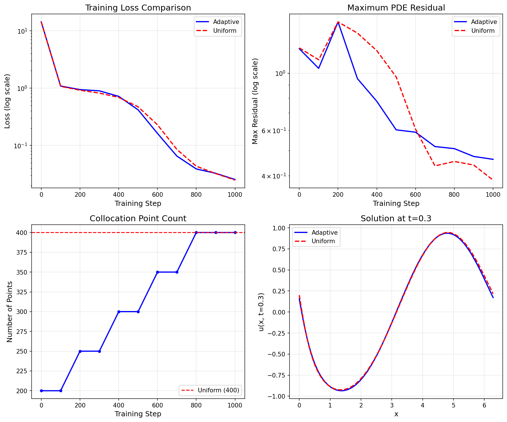
Training Comparison

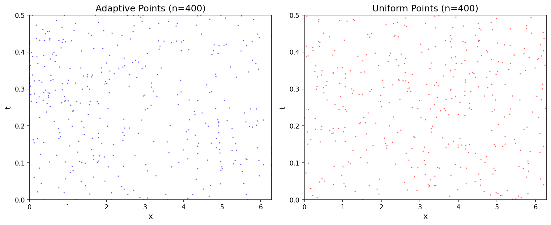
Point Distribution

Results Summary

Both methods use the same total collocation budget (200 points); only the placement differs. Accuracy is measured against the spectral reference solution, not the training loss.

Method	Final Points	Solution Relative L2
Adaptive (RAR-D)	200	0.0749
Uniform	200	0.0821

Key Observations:

• At a tight point budget, adaptive RAR-D reduces the solution error by ~9% over uniform with the same number of points — it concentrates the scarce points on the steep travelling front where uniform sampling under-resolves.
• The meaningful comparison is solution error against a reference, not training loss on each method's own (different) collocation points.
• The advantage grows when points are scarce relative to the localized feature; with a very dense uniform grid the gap shrinks.

Next Steps

Experiments to Try

1. Increase refinement: Add more points per step
2. Lower beta: Smoother probability distribution (beta < 1)
3. Higher beta: Sharper focus on max residual (beta > 1)
4. Sharper shocks: Reduce viscosity to see adaptive benefit

Related Examples

• NTK Analysis - Diagnose training dynamics
• GradNorm - Balance loss components
• Burgers PINN - Basic Burgers equation

API Reference

• RARDRefiner
• RARDConfig
• solve_burgers_spectral

Troubleshooting

Points clustering too tightly

• Increase noise_scale in RARDConfig
• Lower percentile_threshold to spread refinement
• Lower beta for smoother probability distribution

Not enough refinement

• Increase num_new_points
• Decrease refine_frequency
• Raise percentile_threshold to be more selective

Points leaving domain

• Check bounds are correct: bounds = jnp.array([[x_min, x_max], [t_min, t_max]])
• Refinement clips to bounds automatically

Memory growing too fast

• Cap maximum number of points
• Tune percentile_threshold / num_new_points to trade concentration vs coverage
• Consider periodic pruning of low-residual points