Inverse Diffusion Equation PINN¶

Metadata	Value
Level	Advanced
Runtime	~3 min (GPU) / ~15 min (CPU)
Prerequisites	JAX, Flax NNX, inverse problems
Format	Python + Jupyter
Memory	~500 MB RAM

Overview¶

This tutorial demonstrates solving an inverse problem: discovering the unknown diffusion coefficient in the heat/diffusion equation from sparse observations. This is a fundamental inverse problem in PDE parameter identification.

Inverse problems are critical for scientific applications where model parameters are unknown but observations of the system are available. PINNs provide a natural framework for these problems by treating the unknown parameter as a trainable variable.

What You'll Learn¶

Implement a PINN with trainable PDE parameters
Design loss functions for inverse problems
Balance physics constraints with observation data
Track parameter convergence during training
Validate discovered parameters against ground truth

Coming from DeepXDE?¶

DeepXDE	Opifex (JAX)
`dde.Variable(2.0)`	`nnx.Param(jnp.log(jnp.array(C_init)))`
`external_trainable_variables=C`	Parameter included in `nnx.Param` state
`dde.callbacks.VariableValue(C)`	Track `pinn.C` directly in training loop
`model.train(iterations=50000)`	20000 epochs with Adam optimizer

Key differences:

Log transform: Use log_C with exp to ensure positivity
Native tracking: Parameter history tracked directly without callbacks
Unified optimization: Both network and parameter use same optimizer

Files¶

Python Script: examples/pinns/inverse_diffusion.py
Jupyter Notebook: examples/pinns/inverse_diffusion.ipynb

Quick Start¶

Run the Python Script¶

source activate.sh && python examples/pinns/inverse_diffusion.py

Run the Jupyter Notebook¶

jupyter lab examples/pinns/inverse_diffusion.ipynb

Core Concepts¶

Inverse Problem Formulation¶

Forward problem: Given the PDE parameters, solve for the solution.

Inverse problem: Given observations, discover the unknown parameters.

\[\frac{\partial u}{\partial t} - C \frac{\partial^2 u}{\partial x^2} + f(x, t) = 0\]

Component	This Example
Domain	\(x \in [-1, 1]\), \(t \in [0, 1]\)
Unknown	Diffusion coefficient \(C\) (true value = 1.0)
Initial guess	\(C = 2.0\)
Observations	10 points at \(t = 1\)
Exact solution	\(u(x, t) = \sin(\pi x) e^{-t}\)

Why Inverse Problems are Challenging¶

Ill-posedness: Small changes in data can cause large parameter changes
Non-uniqueness: Multiple parameters may fit the same observations
Noise sensitivity: Real observations include measurement noise
Regularization: May be needed to stabilize the solution

Implementation¶

Step 1: Imports and Configuration¶

import jax
import jax.numpy as jnp
import optax
from flax import nnx

Terminal Output:

======================================================================
Opifex Example: Inverse Diffusion Equation PINN
======================================================================
JAX backend: gpu
JAX devices: [CudaDevice(id=0)]

True diffusion coefficient: C = 1.0
Domain: x in [-1.0, 1.0], t in [0.0, 1.0]
Collocation: 400 domain, 100 boundary, 100 initial
Observation points: 10 at t=1 (for parameter discovery)
Network: [2] + [32, 32, 32] + [1]
Training: 20000 epochs @ lr=0.001

Step 2: Define the Problem¶

C_TRUE = 1.0  # True value to be discovered

def exact_solution(x, t):
    """Exact solution: u(x, t) = sin(pi*x) * exp(-t)."""
    return jnp.sin(jnp.pi * x) * jnp.exp(-t)

def source_term(x, t):
    """Source term f(x, t) computed from exact solution."""
    return jnp.exp(-t) * (jnp.sin(jnp.pi * x) - jnp.pi**2 * jnp.sin(jnp.pi * x))

Terminal Output:

Diffusion equation: du/dt - C * d^2u/dx^2 = f(x, t)
  True coefficient: C = 1.0
  Exact solution: u(x, t) = sin(pi*x) * exp(-t)
  BC: u(-1, t) = u(1, t) = 0
  IC: u(x, 0) = sin(pi*x)
  Goal: Discover C from sparse observations at t=1

Step 3: Create PINN with Trainable Parameter¶

class InverseDiffusionPINN(nnx.Module):
    def __init__(self, hidden_dims: list[int], C_init: float, *, rngs: nnx.Rngs):
        super().__init__()

        # Trainable diffusion coefficient (to be discovered)
        # Use log transform to ensure positivity
        self.log_C = nnx.Param(jnp.log(jnp.array(C_init)))

        layers = []
        in_features = 2  # (x, t)

        for hidden_dim in hidden_dims:
            layers.append(nnx.Linear(in_features, hidden_dim, rngs=rngs))
            in_features = hidden_dim

        layers.append(nnx.Linear(in_features, 1, rngs=rngs))
        self.layers = nnx.List(layers)

    @property
    def coef(self) -> jax.Array:
        """Return positive diffusion coefficient via exp transform."""
        return jnp.exp(self.log_C.value)

    def __call__(self, xt: jax.Array) -> jax.Array:
        h = xt
        for layer in self.layers[:-1]:
            h = jnp.tanh(layer(h))
        return self.layers[-1](h)

# Initialize with incorrect guess (C=2.0, true is C=1.0)
pinn = InverseDiffusionPINN(hidden_dims=[32, 32, 32], C_init=2.0, rngs=nnx.Rngs(42))

Terminal Output:

Creating PINN model...
PINN parameters: 2,242
Initial C guess: 2.000000
True C:          1.000000

Step 4: Generate Collocation and Observation Points¶

key = jax.random.PRNGKey(42)
keys = jax.random.split(key, 6)

# Domain interior points
xt_domain = jnp.column_stack([x_domain, t_domain])

# Boundary and initial condition points
xt_bc = jnp.vstack([xt_bc_left, xt_bc_right])
u_bc = exact_solution(xt_bc[:, 0], xt_bc[:, 1])

xt_ic = jnp.column_stack([x_ic, jnp.zeros(N_INITIAL)])
u_ic = exact_solution(x_ic, jnp.zeros(N_INITIAL))

# Observation points at t=1 (key for parameter discovery)
x_obs = jnp.linspace(X_MIN, X_MAX, N_OBSERVE)
t_obs = jnp.ones(N_OBSERVE)
xt_obs = jnp.column_stack([x_obs, t_obs])
u_obs = exact_solution(x_obs, t_obs)

Terminal Output:

Generating collocation points and observations...
Domain points:      (400, 2)
Boundary points:    (100, 2)
Initial points:     (100, 2)
Observation points: (10, 2) (at t=1)

Step 5: Define Physics-Informed Loss¶

def compute_pde_residual(pinn, xt):
    """Compute diffusion PDE residual: u_t - C*u_xx + f = 0."""

    def u_scalar(xt_single):
        return pinn(xt_single.reshape(1, 2)).squeeze()

    def residual_single(xt_single):
        x, t = xt_single[0], xt_single[1]
        grad_u = jax.grad(u_scalar)(xt_single)
        u_t = grad_u[1]
        hess = jax.hessian(u_scalar)(xt_single)
        u_xx = hess[0, 0]
        f = source_term(x, t)
        # Use pinn.coef (the trainable parameter)
        return u_t - pinn.coef * u_xx + f

    return jax.vmap(residual_single)(xt)

def data_loss(pinn, xt, u_target):
    """Loss from observation data - key for parameter discovery."""
    u = pinn(xt).squeeze()
    return jnp.mean((u - u_target) ** 2)

def total_loss(pinn, xt_dom, xt_bc, u_bc, xt_ic, u_ic, xt_obs, u_obs):
    """Total loss = PDE + BC + IC + Data fitting."""
    return pde_loss(pinn, xt_dom) + bc_loss(pinn, xt_bc, u_bc) \
           + ic_loss(pinn, xt_ic, u_ic) + data_loss(pinn, xt_obs, u_obs)

Step 6: Training¶

opt = nnx.Optimizer(pinn, optax.adam(LEARNING_RATE), wrt=nnx.Param)

@nnx.jit
def train_step(pinn, opt, xt_dom, xt_bc, u_bc, xt_ic, u_ic, xt_obs, u_obs):
    def loss_fn(model):
        return total_loss(model, xt_dom, xt_bc, u_bc, xt_ic, u_ic, xt_obs, u_obs)

    loss, grads = nnx.value_and_grad(loss_fn)(pinn)
    opt.update(pinn, grads)
    return loss

for epoch in range(EPOCHS):
    loss = train_step(pinn, opt, xt_domain, xt_bc, u_bc, xt_ic, u_ic, xt_obs, u_obs)
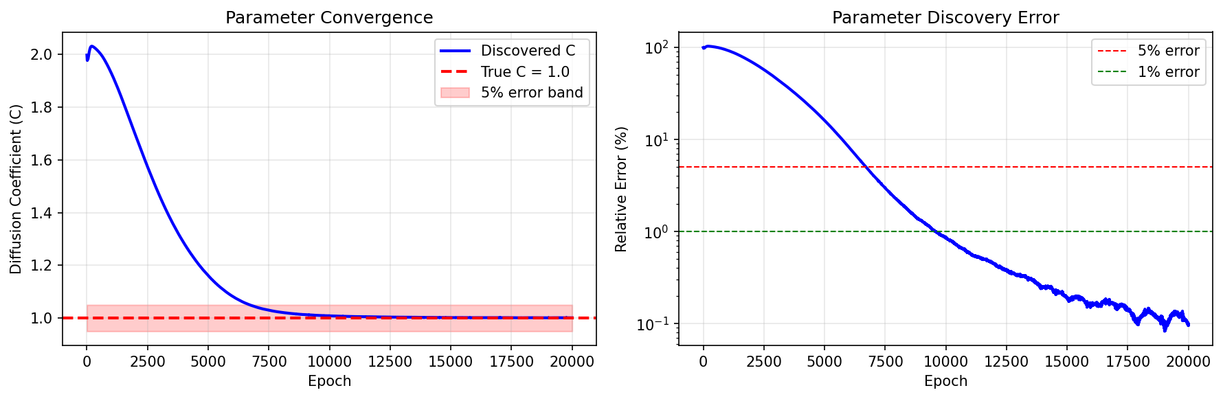
    C_history.append(float(pinn.coef))

Terminal Output:

Training PINN (discovering diffusion coefficient)...
  Epoch     1/20000: loss=4.636221e+01, C=1.998001
  Epoch  4000/20000: loss=5.187262e-03, C=1.284711
  Epoch  8000/20000: loss=1.486299e-04, C=1.022007
  Epoch 12000/20000: loss=7.019506e-05, C=1.004451
  Epoch 16000/20000: loss=2.005360e-04, C=1.001598
  Epoch 20000/20000: loss=5.279011e-05, C=1.000966
Final loss: 5.279011e-05

Discovered C: 1.000966
True C:       1.000000
Relative error: 0.10%

Step 7: Evaluation¶

Terminal Output:

Evaluating PINN...
Relative L2 error:   2.862643e-03
Maximum point error: 4.653510e-03
Mean point error:    1.126259e-03
Mean PDE residual:   5.042705e-03

Visualization¶

Inverse Diffusion Solution

Parameter Convergence Analysis

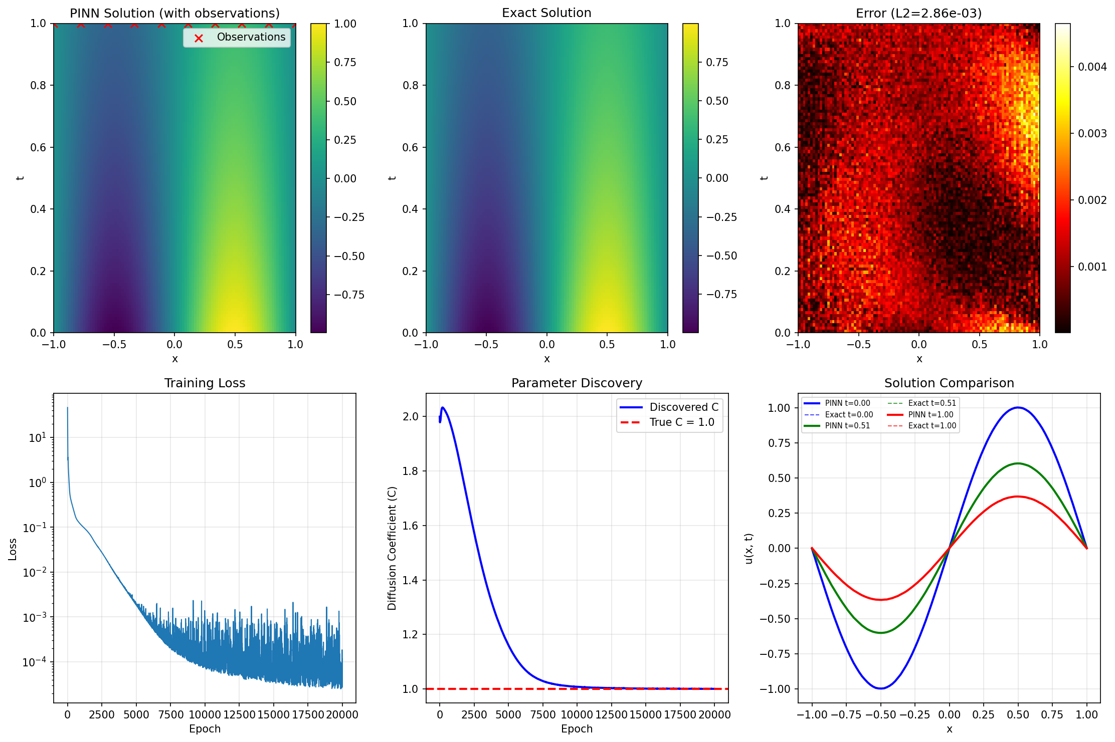
Results Summary¶

Metric	Value
Final Loss	5.28e-05
Discovered C	1.000966
True C	1.000000
Parameter Error	0.10%
Relative L2 Error	0.29%
Mean Point Error	1.13e-03
Mean PDE Residual	5.04e-03
Parameters	2,242
Training Epochs	20,000

Next Steps¶

Experiments to Try¶

Add noise: Corrupt observations with Gaussian noise to test robustness
Fewer observations: Try 5 or 3 observation points
Different initial guess: Start from C=0.1 or C=10.0
Multiple parameters: Discover both C and a reaction coefficient
Real data: Apply to experimental measurements

Example	Level	What You'll Learn
Heat Equation	Beginner	Forward diffusion problem
Burgers Equation	Intermediate	Forward nonlinear problem
Poisson Equation	Beginner	Elliptic PDE (no time)

Troubleshooting¶

Issue	Solution
Parameter diverges	Check PDE residual sign; ensure source term matches
Slow convergence	Increase observation weight or add more observations
Parameter oscillates	Reduce learning rate or use learning rate scheduling
Wrong convergence	Verify exact solution and source term are consistent

API Reference¶

nnx.Param: Flax NNX trainable parameter
jax.grad: Automatic differentiation for PDE derivatives
jax.hessian: Second-order derivatives for diffusion term

Inverse Diffusion Equation PINN¶

Overview¶

What You'll Learn¶

Coming from DeepXDE?¶

Files¶

Quick Start¶

Run the Python Script¶

Run the Jupyter Notebook¶

Core Concepts¶

Inverse Problem Formulation¶

Why Inverse Problems are Challenging¶

Implementation¶

Step 1: Imports and Configuration¶

Step 2: Define the Problem¶

Step 3: Create PINN with Trainable Parameter¶

Step 4: Generate Collocation and Observation Points¶

Step 5: Define Physics-Informed Loss¶

Step 6: Training¶

Step 7: Evaluation¶

Visualization¶

Results Summary¶

Next Steps¶

Experiments to Try¶

Related Examples¶

Troubleshooting¶

API Reference¶