Bayesian FNO on Darcy Flow

Metadata	Value
Level	Intermediate
Runtime	~2 min (GPU) / ~10 min (CPU)
Prerequisites	JAX, Flax NNX, Deep Ensembles
Format	Python + Jupyter
Memory	~2 GB RAM

Overview

This example quantifies predictive uncertainty for the Darcy permeability-to-pressure operator with a heteroscedastic deep ensemble of Fourier Neural Operators. Each member is a ProbabilisticFourierNeuralOperator — an FNO backbone with twin pointwise heads that emit a per-location mean and log-variance. Training each member by the heteroscedastic-Gaussian negative log-likelihood gives the aleatoric axis (input-dependent noise); the disagreement across members gives the epistemic axis (model uncertainty). Their sum is the total predictive variance.

Key Concepts:

• Deep Ensemble: Independently-trained members; their spread is the epistemic (model) uncertainty (Lakshminarayanan et al. 2017).
• Heteroscedastic Head: Each member predicts a per-location variance, the aleatoric (data) uncertainty (Kendall & Gal 2017).
• Variance Calibration: A single positive scale, fit on a held-out split, aligns the predictive std with the observed error spread.

What You'll Learn

1. Build a heteroscedastic FNO with ProbabilisticFourierNeuralOperator
2. Train an ensemble with the heteroscedastic-Gaussian NLL loss
3. Decompose predictive variance into aleatoric + epistemic parts
4. Calibrate and visualize the predictive uncertainty

Coming from Standard FNO?

Standard FNO	Bayesian FNO (This Example)
Point predictions	Predictive mean + calibrated std
model(x) returns y	Member returns (mean, log_variance)
Relative-L2 loss	Heteroscedastic-Gaussian NLL
No uncertainty	Aleatoric + epistemic decomposition

Key differences:

1. Ensemble: Several independently-seeded members vote on the answer.
2. Variance head: Each member learns an input-dependent noise level.
3. Calibration: One held-out scale aligns the interval with coverage.

Files

• Python Script: examples/uncertainty/bayesian_fno.py
• Jupyter Notebook: examples/uncertainty/bayesian_fno.ipynb

Quick Start

Run the Python Script

source activate.sh && python examples/uncertainty/bayesian_fno.py

Run the Jupyter Notebook

jupyter lab examples/uncertainty/bayesian_fno.ipynb

Core Concepts

Heteroscedastic Deep Ensemble

Each member predicts a per-location Gaussian N(mu(x), sigma^2(x)). The ensemble decomposes the total predictive variance as

total = aleatoric + epistemic
      = mean_m[sigma_m^2(x)] + var_m[mu_m(x)]

where m indexes ensemble members. The aleatoric term captures input-dependent noise; the epistemic term captures member disagreement.

Components

Component	Role
ProbabilisticFourierNeuralOperator	FNO backbone + mean / log-variance heads
probabilistic_fno_negative_log_likelihood	Heteroscedastic-Gaussian training loss
append_grid_coordinates	Positional embedding (boundary-value problems)
ensemble_predictive	Aggregates member means into the epistemic spread

Implementation

Step 1: Build a Heteroscedastic Member

The backbone is translation-equivariant, so grid-coordinate channels are prepended to the input — each member is built with in_channels = 1 + 2.

from opifex.neural.operators.fno.probabilistic import (
    ProbabilisticFourierNeuralOperator,
)

member = ProbabilisticFourierNeuralOperator(
    in_channels=3,  # 1 permeability + 2 grid coordinates
    out_channels=1,
    hidden_channels=32,
    modes=12,
    num_layers=4,
    rngs=nnx.Rngs(42),
)

Terminal Output:

Creating heteroscedastic FNO ensemble...
  Member: ProbabilisticFNO (modes=12, width=32, layers=4)
  Input channels: 1 (+ 2 grid = 3)
  Parameters per member: 2,372,066
  Ensemble parameters:   9,488,264

Step 2: Train the Ensemble

Every member is trained independently with the heteroscedastic-Gaussian NLL on grid-augmented, Gaussian-normalized inputs.

from opifex.neural.operators.fno._positional import append_grid_coordinates
from opifex.neural.operators.fno.probabilistic import (
    probabilistic_fno_negative_log_likelihood,
)


@nnx.jit
def train_step(member, optimizer, x, y):
    def loss_fn(model):
        return probabilistic_fno_negative_log_likelihood(
            model, append_grid_coordinates(x), y
        )

    loss, grads = nnx.value_and_grad(loss_fn)(member)
    optimizer.update(member, grads)
    return loss

Terminal Output:

Training ensemble members...
  Member 1/4: NLL +0.7451 -> -2.9116
  Member 2/4: NLL +0.6524 -> -1.3052
  Member 3/4: NLL +0.5145 -> -2.3262
  Member 4/4: NLL +0.4694 -> -2.2192
Training time: 63.4s

Step 3: Predict and Calibrate

The predictive mean and aleatoric + epistemic variance are assembled in physical units, then a single scale is fit on a held-out calibration split so the 1.64-sigma interval covers ~90% of the residuals.

Terminal Output:

Calibrating predictive uncertainty...
  Calibration std scale: 0.2316

Evaluating on test set...

Results:
  Predictive-mean Relative L2: 0.009013
  Min / Max Relative L2:       0.003607 / 0.023608
  Test MSE:                    6.115206e-06
  Mean predictive std:         2.180397e-03
  Mean aleatoric std:          9.141234e-03
  Mean epistemic std:          2.010190e-03

Step 4: Calibration Analysis

Terminal Output:

Uncertainty calibration analysis...
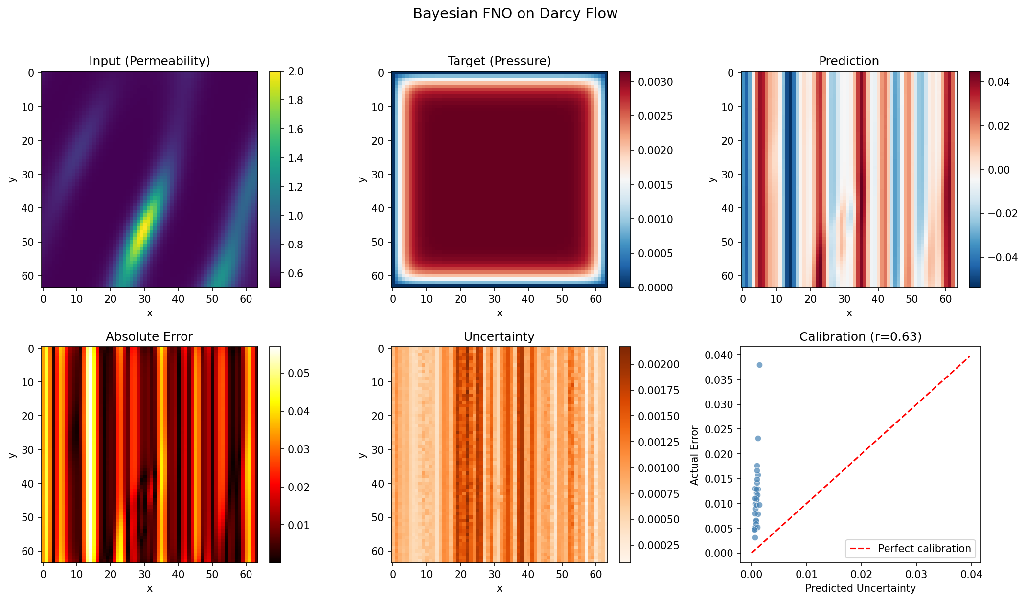
  Coverage @ 1.64-sigma: 87.8% (target 90%)
  1-sigma coverage:           66.3%
  2-sigma coverage:           93.4%
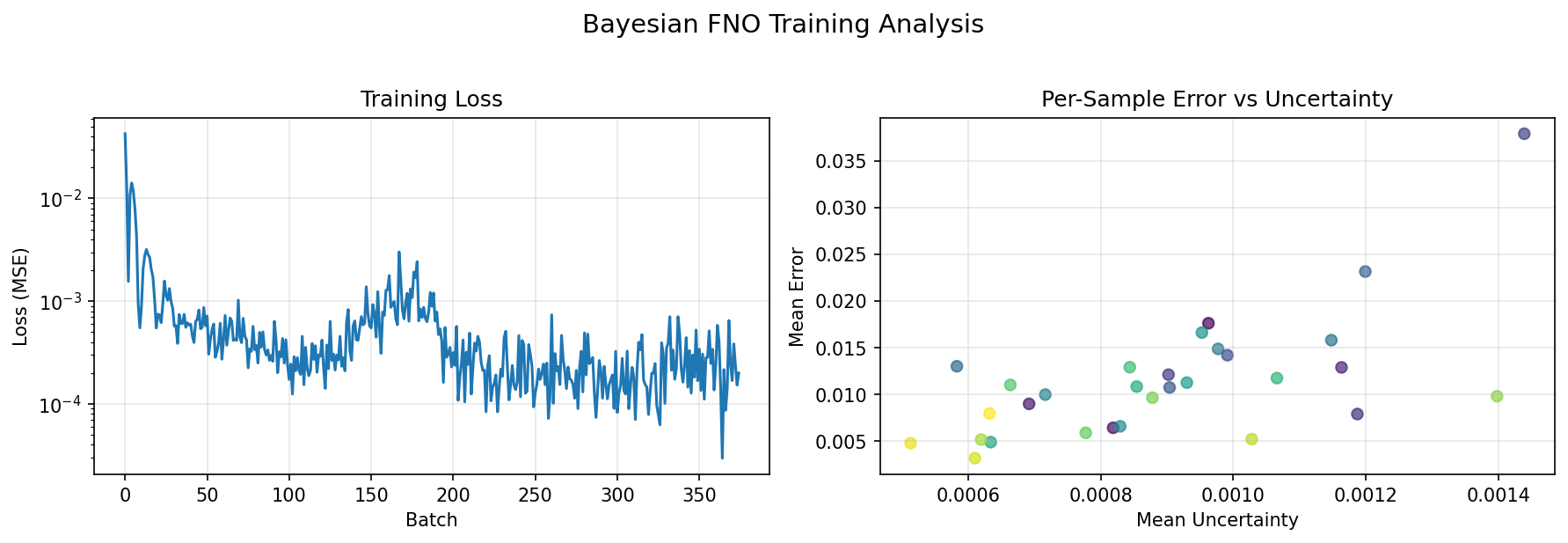
  Error-uncertainty corr (per-sample): 0.1709
  Error-uncertainty corr (per-pixel):  0.3546

Visualization

Results Summary

Metric	Value
Predictive-mean Relative L2	0.009013
Min / Max Relative L2	0.003607 / 0.023608
Coverage @ 1.64-sigma	87.8%
2-sigma coverage	93.4%
Error-uncertainty corr (per-sample)	0.1709
Error-uncertainty corr (per-pixel)	0.3546
Parameters per member	2,372,066
Ensemble parameters	9,488,264
Training time	~63s

The predictive mean visually matches the smooth ground-truth pressure field, and the calibrated predictive std is larger where the absolute error is larger — an actionable, well-calibrated risk signal.

Next Steps

Experiments to Try

1. More members: Increase NUM_MEMBERS for a smoother epistemic estimate (diminishing returns past ~5 on this smooth dataset).
2. Higher capacity: Raise MODES / HIDDEN_WIDTH for sharper means.
3. Target coverage: Change TARGET_COVERAGE to calibrate a different predictive interval (e.g. 0.95).
4. Different backbones: Swap the member backbone for TFNO or UNO and keep the same heteroscedastic-ensemble wrapper.

Related Examples

Example	Level	What You'll Learn
UQNO on Darcy	Intermediate	Built-in Bayesian convolutions
FNO on Darcy	Beginner	Standard FNO training
Calibration Methods	Intermediate	Post-hoc calibration

API Reference

• ProbabilisticFourierNeuralOperator: FNO with mean + log-variance heads
• probabilistic_fno_negative_log_likelihood: Heteroscedastic-Gaussian NLL
• append_grid_coordinates: Grid positional embedding
• ensemble_predictive: Member-aggregation predictive constructor

Troubleshooting

Issue	Solution
Over-confident intervals	The held-out variance scale corrects this; widen the calibration split if it is noisy
Out-of-memory on evaluation	Lower EVAL_CHUNK
Weak per-sample correlation	Train members longer or reduce per-member capacity for more diversity

Notes

This example uses a heteroscedastic deep ensemble: each member is a ProbabilisticFourierNeuralOperator trained by the heteroscedastic-Gaussian NLL, and the predictive variance is the standard aleatoric + epistemic decomposition, calibrated to the target coverage on a held-out split. This is the canonical scalable Bayesian-predictive recipe and it preserves the operator-learning accuracy of a deterministic FNO.