Diffusion-Reaction Equation PINN¶

Metadata	Value
Level	Intermediate
Runtime	~3 min (GPU) / ~12 min (CPU)
Prerequisites	JAX, Flax NNX, PDEs
Format	Python + Jupyter
Memory	~500 MB RAM

Overview¶

This tutorial demonstrates solving a diffusion-reaction equation using a PINN. The problem features multiple frequency components (sine waves) that the network must learn simultaneously, making it a good test for spectral approximation.

The equation models phenomena where diffusion and source/reaction terms compete, such as heat transfer with internal heat generation or chemical diffusion with reaction kinetics.

What You'll Learn¶

Implement a PINN for diffusion-reaction PDEs
Apply hard constraints for multi-frequency initial conditions
Handle manufactured solutions with complex source terms
Understand how networks learn multiple frequency components

Coming from DeepXDE?¶

DeepXDE	Opifex (JAX)
`dde.geometry.Interval(-np.pi, np.pi)`	`jnp.linspace(-jnp.pi, jnp.pi, N)`
`net.apply_output_transform(transform)`	Hard constraint in `__call__` method
`dde.nn.FNN([2] + [30]*6 + [1])`	`nnx.Linear` layers with tanh activation
`model.train(iterations=20000)`	15000 epochs with Adam optimizer

Key differences:

Hard constraint: u = t*(pi^2 - x^2)*u_hat + IC(x) enforces IC and BC
Source term: Computed analytically from manufactured solution
Multi-frequency IC: Sum of sin(kx)/k terms with k = 1, 2, 3, 4, 8

Files¶

Python Script: examples/pinns/diffusion_reaction.py
Jupyter Notebook: examples/pinns/diffusion_reaction.ipynb

Quick Start¶

Run the Python Script¶

source activate.sh && python examples/pinns/diffusion_reaction.py

Run the Jupyter Notebook¶

jupyter lab examples/pinns/diffusion_reaction.ipynb

Core Concepts¶

Diffusion-Reaction Equation¶

\[\frac{\partial u}{\partial t} = D \frac{\partial^2 u}{\partial x^2} + f(x, t)\]

Component	This Example
Domain	\(x \in [-\pi, \pi]\), \(t \in [0, 1]\)
Diffusion	\(D = 1\)
Solution	\(u = e^{-t}(\sin x + \frac{\sin 2x}{2} + \frac{\sin 3x}{3} + \frac{\sin 4x}{4} + \frac{\sin 8x}{8})\)
IC	Sum of sine waves at \(t=0\)
BC	\(u(\pm\pi, t) = 0\) (Dirichlet)

Physical Interpretation¶

Diffusion: Smooths spatial gradients
Source term: Chosen to maintain the multi-frequency structure
Exponential decay: All frequency components decay at the same rate

Implementation¶

Step 1: Imports and Configuration¶

import jax
import jax.numpy as jnp
import optax
from flax import nnx

Terminal Output:

======================================================================
Opifex Example: Diffusion-Reaction Equation PINN
======================================================================
JAX backend: gpu
JAX devices: [CudaDevice(id=0)]

Diffusion coefficient: D = 1.0
Domain: x in [-3.1416, 3.1416], t in [0.0, 1.0]
Collocation: 2000 domain, 100 boundary, 200 initial
Network: [2] + [30, 30, 30, 30, 30, 30] + [1]
Training: 15000 epochs @ lr=0.001

Step 2: Define the Problem¶

D = 1.0  # Diffusion coefficient

def exact_solution(x, t):
    """Exact solution: sum of sine waves with exponential decay."""
    return jnp.exp(-t) * (
        jnp.sin(x) + jnp.sin(2*x)/2 + jnp.sin(3*x)/3
        + jnp.sin(4*x)/4 + jnp.sin(8*x)/8
    )

def source_term(x, t):
    """Source term f(x, t) for the manufactured solution."""
    return jnp.exp(-t) * (
        3*jnp.sin(2*x)/2 + 8*jnp.sin(3*x)/3
        + 15*jnp.sin(4*x)/4 + 63*jnp.sin(8*x)/8
    )

Terminal Output:

Diffusion-reaction: du/dt = D*d^2u/dx^2 + f(x,t)
  Diffusion: D = 1.0
  Solution: sum of sin(kx)/k terms with exp(-t) decay
  BC: u(-pi, t) = u(pi, t) = 0 (periodic-like)
  IC: u(x, 0) = sin(x) + sin(2x)/2 + ...

Step 3: Create PINN with Hard Constraint¶

class DiffusionReactionPINN(nnx.Module):
    def __init__(self, hidden_dims: list[int], *, rngs: nnx.Rngs):
        super().__init__()
        layers = []
        in_features = 2  # (x, t)

        for hidden_dim in hidden_dims:
            layers.append(nnx.Linear(in_features, hidden_dim, rngs=rngs))
            in_features = hidden_dim

        layers.append(nnx.Linear(in_features, 1, rngs=rngs))
        self.layers = nnx.List(layers)

    def __call__(self, xt: jax.Array) -> jax.Array:
        """Forward pass with hard constraint for IC and BC."""
        x, t = xt[:, 0:1], xt[:, 1:2]

        # Network output
        h = xt
        for layer in self.layers[:-1]:
            h = jnp.tanh(layer(h))
        u_hat = self.layers[-1](h)

        # Hard constraint: u = t*(pi^2 - x^2)*u_hat + IC(x)
        ic_term = (jnp.sin(x) + jnp.sin(2*x)/2 + jnp.sin(3*x)/3
                   + jnp.sin(4*x)/4 + jnp.sin(8*x)/8)
        bc_mask = t * (jnp.pi**2 - x**2)

        return bc_mask * u_hat + ic_term

pinn = DiffusionReactionPINN(hidden_dims=[30]*6, rngs=nnx.Rngs(42))

Terminal Output:

Creating PINN model...
PINN parameters: 4,771

Step 4: Generate Collocation Points¶

key = jax.random.PRNGKey(42)
keys = jax.random.split(key, 4)

# Domain interior points
x_domain = jax.random.uniform(keys[0], (N_DOMAIN,), minval=X_MIN, maxval=X_MAX)
t_domain = jax.random.uniform(keys[1], (N_DOMAIN,), minval=T_MIN, maxval=T_MAX)
xt_domain = jnp.column_stack([x_domain, t_domain])

Terminal Output:

Generating collocation points...
Domain points: (2000, 2)

Step 5: Define Physics-Informed Loss¶

def compute_pde_residual(pinn, xt):
    """Compute diffusion-reaction PDE residual."""

    def u_scalar(xt_single):
        return pinn(xt_single.reshape(1, 2)).squeeze()

    def residual_single(xt_single):
        x, t = xt_single[0], xt_single[1]

        grad_u = jax.grad(u_scalar)(xt_single)
        u_t = grad_u[1]

        hess = jax.hessian(u_scalar)(xt_single)
        u_xx = hess[0, 0]

        f = source_term(x, t)

        # Residual: u_t - D*u_xx - f = 0
        return u_t - D * u_xx - f

    return jax.vmap(residual_single)(xt)

def pde_loss(pinn, xt):
    residual = compute_pde_residual(pinn, xt)
    return jnp.mean(residual**2)

Step 6: Training¶

opt = nnx.Optimizer(pinn, optax.adam(LEARNING_RATE), wrt=nnx.Param)

@nnx.jit
def train_step(pinn, opt, xt_dom):
    def loss_fn(model):
        return pde_loss(model, xt_dom)

    loss, grads = nnx.value_and_grad(loss_fn)(pinn)
    opt.update(pinn, grads)
    return loss

for epoch in range(EPOCHS):
    loss = train_step(pinn, opt, xt_domain)

Terminal Output:

Training PINN...
  Epoch     1/15000: loss=2.404716e+01
  Epoch  3000/15000: loss=8.812878e-03
  Epoch  6000/15000: loss=4.998077e-03
  Epoch  9000/15000: loss=7.960054e-03
  Epoch 12000/15000: loss=1.765104e-03
  Epoch 15000/15000: loss=5.911256e-03
Final loss: 5.911256e-03

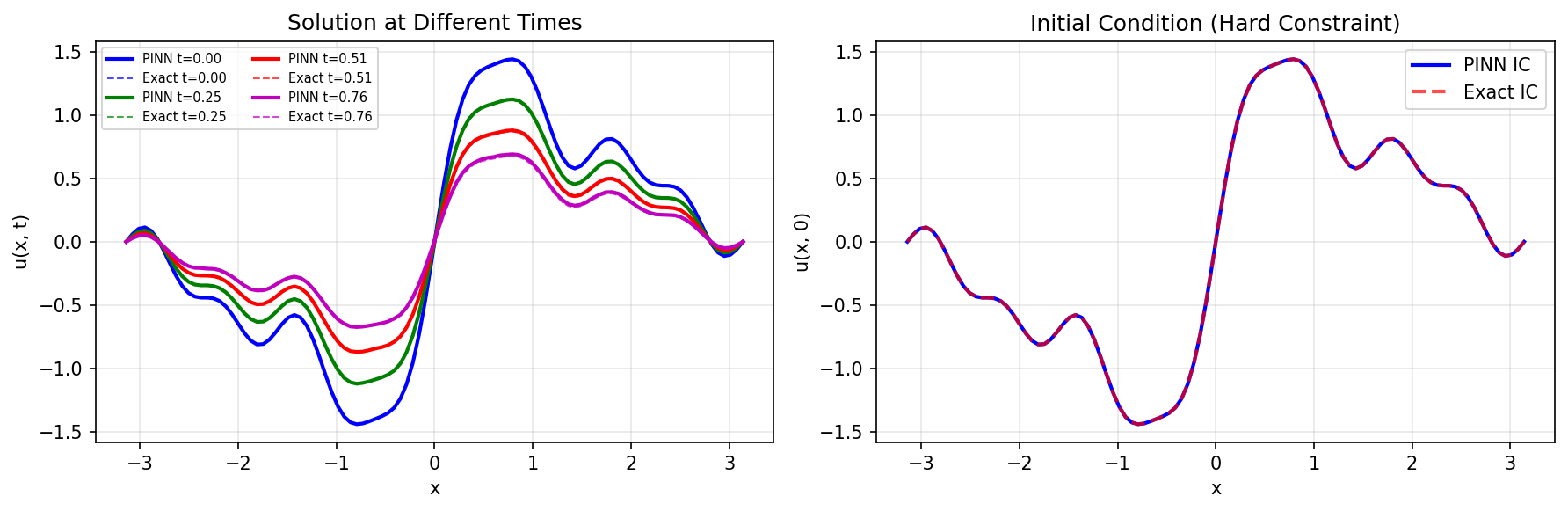
Step 7: Evaluation¶

Terminal Output:

Evaluating PINN...
Relative L2 error:   1.364888e-02
Maximum point error: 2.670667e-02
Mean point error:    5.508810e-03
Mean PDE residual:   5.571126e-02
IC error (hard):     0.000000e+00

Visualization¶

Diffusion-Reaction Solution

Analysis

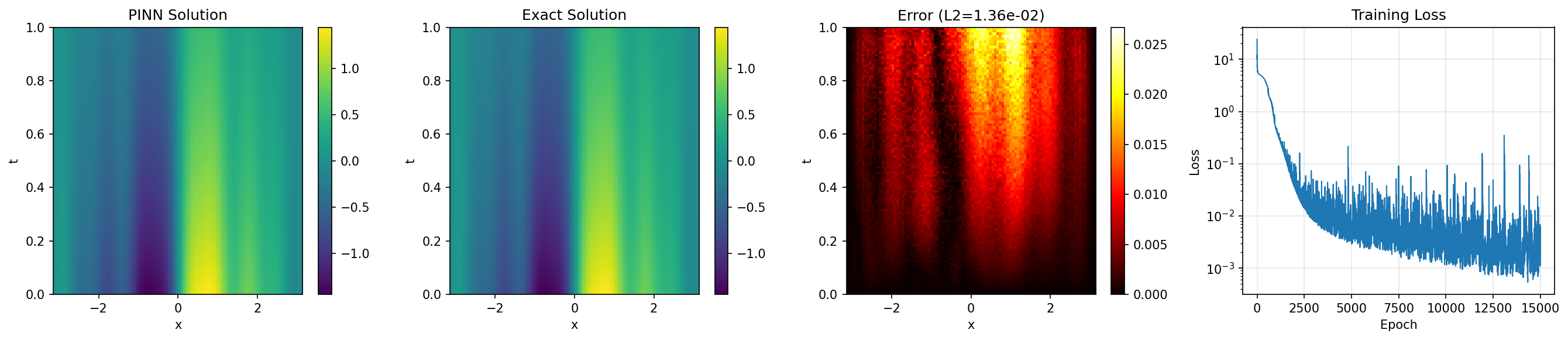
Results Summary¶

Metric	Value
Final Loss	5.91e-03
Relative L2 Error	1.36%
Maximum Error	2.67e-02
Mean PDE Residual	5.57e-02
IC Error (hard)	0.0
Parameters	4,771
Training Epochs	15,000

Next Steps¶

Experiments to Try¶

Fewer frequencies: Remove higher frequency terms to see easier convergence
More epochs: Train for 30000+ epochs to reduce residual
Larger network: Try [40]*8 for better frequency resolution
Different decay: Modify source term for non-uniform decay rates

Example	Level	What You'll Learn
Heat Equation	Beginner	Simpler diffusion (no reaction)
Allen-Cahn	Advanced	Nonlinear reaction term
Helmholtz	Intermediate	Multi-frequency with sin act

Troubleshooting¶

Issue	Solution
High frequency not captured	Increase network depth or width
IC not exact	Check hard constraint formula matches exact IC
Slow convergence	Try learning rate scheduling
Loss oscillates	Reduce learning rate or add more collocation points

Diffusion-Reaction Equation PINN¶

Overview¶

What You'll Learn¶

Coming from DeepXDE?¶

Files¶

Quick Start¶

Run the Python Script¶

Run the Jupyter Notebook¶

Core Concepts¶

Diffusion-Reaction Equation¶

Physical Interpretation¶

Implementation¶

Step 1: Imports and Configuration¶

Step 2: Define the Problem¶

Step 3: Create PINN with Hard Constraint¶

Step 4: Generate Collocation Points¶

Step 5: Define Physics-Informed Loss¶

Step 6: Training¶

Step 7: Evaluation¶

Visualization¶

Results Summary¶

Next Steps¶

Experiments to Try¶

Related Examples¶

Troubleshooting¶