Navier-Stokes PINN: Kovasznay Flow¶

Metadata	Value
Level	Advanced
Runtime	~8 min (GPU) / ~30 min (CPU)
Prerequisites	JAX, Flax NNX, fluid mechanics
Format	Python + Jupyter
Memory	~1 GB RAM

Overview¶

This tutorial demonstrates solving the 2D steady incompressible Navier-Stokes equations using a Physics-Informed Neural Network (PINN). The Kovasznay flow is an exact analytical solution to Navier-Stokes, making it an ideal benchmark for validating numerical methods.

The Navier-Stokes equations describe the motion of viscous fluids and are fundamental to computational fluid dynamics. PINNs can solve these equations without mesh generation or explicit discretization, learning the velocity and pressure fields directly from the governing physics.

What You'll Learn¶

Implement a PINN for coupled multi-output PDEs (u, v, p)
Compute mixed derivatives using JAX Jacobian and Hessian
Enforce continuity and momentum equations simultaneously
Validate against analytical Kovasznay flow solution
Visualize velocity vector fields and pressure distributions

Coming from DeepXDE?¶

If you are familiar with the DeepXDE library:

DeepXDE	Opifex (JAX)
`dde.geometry.Rectangle(xmin, xmax)`	`jax.random.uniform(key, (N, 2))` for (x, y)
`dde.grad.jacobian(u, x, i=0, j=0)`	`jax.jacobian(uvp_fn)(xy)[0, 0]` for u_x
`dde.grad.hessian(u, x, component=0, i=0)`	`jax.hessian(u_fn)(xy)[0, 0]` for u_xx
`dde.nn.FNN([2]+[50]*4+[3], "tanh")`	Custom `NavierStokesPINN` with nnx.Linear
`model.compile("adam", lr=1e-3)`	`nnx.Optimizer(pinn, optax.adam(lr), wrt=nnx.Param)`
`model.train(iterations=30000)`	Custom training loop with `@nnx.jit`

Key differences:

Multi-output: Network outputs [u, v, p] as a single 3-channel tensor
Jacobian-based: Use jax.jacobian for efficient first derivatives of all outputs
Coupled PDEs: Momentum and continuity equations share the network output
No L-BFGS: This example uses Adam only; add L-BFGS for better convergence

Files¶

Python Script: examples/pinns/navier_stokes.py
Jupyter Notebook: examples/pinns/navier_stokes.ipynb

Quick Start¶

Run the Python Script¶

source activate.sh && python examples/pinns/navier_stokes.py

Run the Jupyter Notebook¶

jupyter lab examples/pinns/navier_stokes.ipynb

Core Concepts¶

Navier-Stokes Equations¶

The 2D steady incompressible Navier-Stokes equations consist of momentum and continuity:

Momentum (x-direction): $$u \frac{\partial u}{\partial x} + v \frac{\partial u}{\partial y} = -\frac{\partial p}{\partial x} + \frac{1}{Re}\left(\frac{\partial^2 u}{\partial x^2} + \frac{\partial^2 u}{\partial y^2}\right)$$

Momentum (y-direction): $$u \frac{\partial v}{\partial x} + v \frac{\partial v}{\partial y} = -\frac{\partial p}{\partial y} + \frac{1}{Re}\left(\frac{\partial^2 v}{\partial x^2} + \frac{\partial^2 v}{\partial y^2}\right)$$

Continuity: $$\frac{\partial u}{\partial x} + \frac{\partial v}{\partial y} = 0$$

Kovasznay Flow¶

The Kovasznay flow is an exact solution with Re = 20:

Component	Formula
x-velocity	$u = 1 - e^{\lambda x} \cos(2\pi y)$
y-velocity	$v = \frac{\lambda}{2\pi} e^{\lambda x} \sin(2\pi y)$
Pressure	$p = \frac{1}{2}(1 - e^{2\lambda x})$
Lambda	$\lambda = \frac{1}{2\nu} - \sqrt{\frac{1}{4\nu^2} + 4\pi^2}$

Where $\nu = 1/Re = 0.05$ is the kinematic viscosity.

PINN Architecture¶

graph TB
    subgraph Input["Collocation Points"]
        A["Domain Points<br/>(x, y) in Ω"]
        B["Boundary Points<br/>(x, y) on ∂Ω"]
    end

    subgraph PINN["Neural Network (x, y) → [u, v, p]"]
        C["Linear + tanh<br/>50 units"]
        D["Linear + tanh<br/>50 units"]
        E["Linear + tanh<br/>50 units"]
        F["Linear + tanh<br/>50 units"]
        G["Linear<br/>3 units"]
    end

    subgraph Loss["Physics-Informed Loss"]
        H["Momentum-x<br/>|u·u_x + v·u_y + p_x - ν∇²u|²"]
        I["Momentum-y<br/>|u·v_x + v·v_y + p_y - ν∇²v|²"]
        J["Continuity<br/>|u_x + v_y|²"]
        K["BC Loss<br/>|u - u_exact|² + |v - v_exact|² + |p - p_exact|²"]
        L["Total Loss"]
    end

    A --> C --> D --> E --> F --> G
    B --> C
    G --> H
    G --> I
    G --> J
    G --> K
    H --> L
    I --> L
    J --> L
    K --> L

    style H fill:#e3f2fd,stroke:#1976d2
    style I fill:#e8f5e9,stroke:#388e3c
    style J fill:#fff3e0,stroke:#f57c00
    style K fill:#fce4ec,stroke:#c2185b
    style L fill:#f3e5f5,stroke:#7b1fa2

Implementation¶

Step 1: Imports and Configuration¶

import jax
import jax.numpy as jnp
import optax
from flax import nnx

Terminal Output:

======================================================================
Opifex Example: Navier-Stokes PINN (Kovasznay Flow)
======================================================================
JAX backend: gpu
JAX devices: [CudaDevice(id=0)]
Reynolds number: Re = 20
Domain: x in [-0.5, 1.0], y in [-0.5, 1.5]
Collocation: 2601 domain, 400 boundary
Network: [2] + [50, 50, 50, 50] + [3]
Training: 30000 epochs @ lr=0.001

Step 2: Define Analytical Solution¶

RE = 20
NU = 1.0 / RE
LAMBDA = 1.0 / (2.0 * NU) - jnp.sqrt(1.0 / (4.0 * NU**2) + 4.0 * jnp.pi**2)

def u_exact(xy):
    x, y = xy[:, 0], xy[:, 1]
    return 1.0 - jnp.exp(LAMBDA * x) * jnp.cos(2.0 * jnp.pi * y)

def v_exact(xy):
    x, y = xy[:, 0], xy[:, 1]
    return LAMBDA / (2.0 * jnp.pi) * jnp.exp(LAMBDA * x) * jnp.sin(2.0 * jnp.pi * y)

def p_exact(xy):
    x = xy[:, 0]
    return 0.5 * (1.0 - jnp.exp(2.0 * LAMBDA * x))

Terminal Output:

Kovasznay Flow: Steady 2D incompressible Navier-Stokes
  Lambda = -1.810099
  u(x,y) = 1 - exp(lambda*x) * cos(2*pi*y)
  v(x,y) = (lambda/2*pi) * exp(lambda*x) * sin(2*pi*y)
  p(x,y) = 0.5 * (1 - exp(2*lambda*x))

Step 3: Create the PINN¶

class NavierStokesPINN(nnx.Module):
    def __init__(self, hidden_dims: list[int], *, rngs: nnx.Rngs):
        layers = []
        in_features = 2  # (x, y)

        for hidden_dim in hidden_dims:
            layers.append(nnx.Linear(in_features, hidden_dim, rngs=rngs))
            in_features = hidden_dim

        layers.append(nnx.Linear(in_features, 3, rngs=rngs))  # [u, v, p]
        self.layers = nnx.List(layers)

    def __call__(self, xy):
        h = xy
        for layer in self.layers[:-1]:
            h = jnp.tanh(layer(h))
        return self.layers[-1](h)

pinn = NavierStokesPINN(hidden_dims=[50, 50, 50, 50], rngs=nnx.Rngs(42))

Terminal Output:

Creating PINN model...
PINN parameters: 7,953

Step 4: Compute PDE Residuals¶

def compute_pde_residuals(pinn, xy):
    def uvp_scalar(xy_single):
        return pinn(xy_single.reshape(1, 2)).squeeze()

    def residuals_single(xy_single):
        uvp = uvp_scalar(xy_single)
        u, v = uvp[0], uvp[1]

        # First derivatives via Jacobian
        jac = jax.jacobian(uvp_scalar)(xy_single)
        u_x, u_y = jac[0, 0], jac[0, 1]
        v_x, v_y = jac[1, 0], jac[1, 1]
        p_x, p_y = jac[2, 0], jac[2, 1]

        # Second derivatives (Hessian diagonals)
        hess_u = jax.hessian(lambda xy: uvp_scalar(xy)[0])(xy_single)
        hess_v = jax.hessian(lambda xy: uvp_scalar(xy)[1])(xy_single)

        u_xx, u_yy = hess_u[0, 0], hess_u[1, 1]
        v_xx, v_yy = hess_v[0, 0], hess_v[1, 1]

        # Momentum equations
        momentum_x = u * u_x + v * u_y + p_x - (1/RE) * (u_xx + u_yy)
        momentum_y = u * v_x + v * v_y + p_y - (1/RE) * (v_xx + v_yy)

        # Continuity
        continuity = u_x + v_y

        return jnp.array([momentum_x, momentum_y, continuity])

    return jax.vmap(residuals_single)(xy)

Step 5: Training¶

Terminal Output:

Training PINN...
  Epoch     1/30000: loss=5.135920e+00
  Epoch  5000/30000: loss=1.756912e-03
  Epoch 10000/30000: loss=4.721234e-04
  Epoch 15000/30000: loss=1.124221e-03
  Epoch 20000/30000: loss=2.046824e-03
  Epoch 25000/30000: loss=1.094199e-03
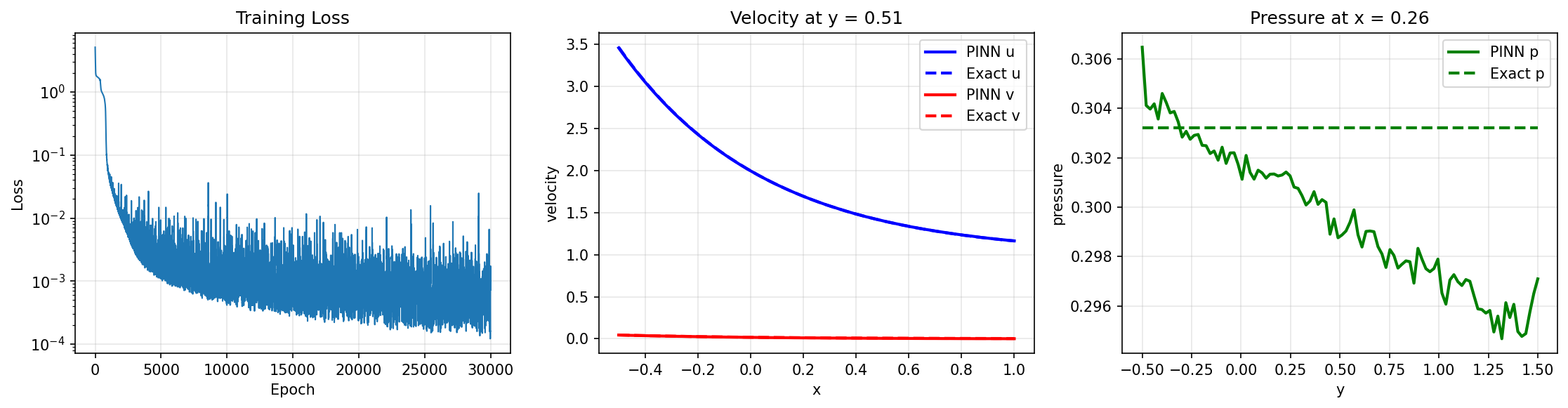
  Epoch 30000/30000: loss=7.266006e-04
Final loss: 7.266006e-04

Step 6: Evaluation¶

Terminal Output:

Evaluating PINN...
L2 relative error (u): 4.457689e-03
L2 relative error (v): 1.126896e-02
L2 relative error (p): 6.496343e-02
Mean PDE residual:     8.192191e-03

Visualization¶

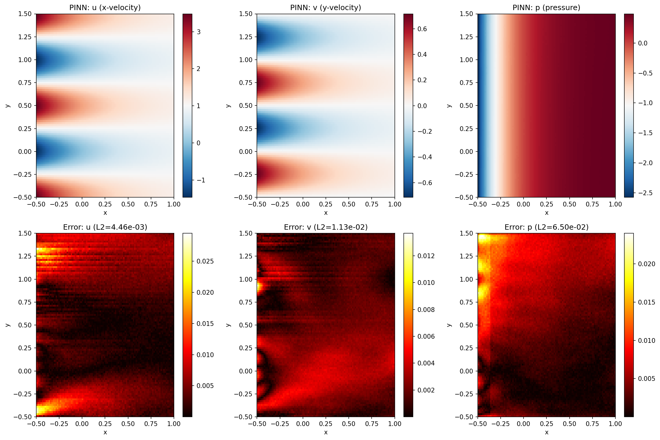
Solution Fields and Errors¶

Navier-Stokes Solution

Training and Cross-Sections¶

Analysis

Results Summary¶

Metric	Value
Final Loss	7.27e-04
L2 Error (u)	0.45%
L2 Error (v)	1.13%
L2 Error (p)	6.50%
Mean PDE Residual	8.19e-03
Parameters	7,953
Training Epochs	30,000

Next Steps¶

Experiments to Try¶

Add L-BFGS: Use optax.lbfgs for second-order refinement
Higher Re: Try Re = 100 or 400 for more challenging flows
More epochs: Train for 50,000+ epochs for better pressure accuracy
Deeper network: Try hidden_dims=[100, 100, 100, 100, 100]
Loss weighting: Balance momentum vs continuity losses

Example	Level	What You'll Learn
Poisson Equation	Intermediate	Simpler elliptic PDE
Burgers Equation	Intermediate	Nonlinear convection
FNO on Darcy Flow	Intermediate	Data-driven alternative
PINO on Burgers	Advanced	Hybrid approach

API Reference¶

nnx.Linear - Linear layer
nnx.Optimizer - Optimizer wrapper
jax.jacobian - Jacobian computation
jax.hessian - Hessian computation

Troubleshooting¶

Pressure error much higher than velocity¶

Symptom: L2 error in p is 5-10x higher than u, v errors.

Cause: Pressure is determined only indirectly through momentum gradients.

Solution: Add pressure reference point constraint or increase BC weighting:

# Fix pressure at a point (e.g., outflow corner)
def pressure_reference_loss(pinn):
    ref_point = jnp.array([[X_MAX, Y_MIN]])
    p_pred = pinn(ref_point)[0, 2]
    p_exact_val = p_exact(ref_point)[0]
    return (p_pred - p_exact_val) ** 2

Loss oscillates without converging¶

Symptom: Loss fluctuates around a value without steady decrease.

Cause: Adam stuck in saddle point or local minimum.

Solution: Add learning rate scheduling or use L-BFGS refinement:

# Learning rate schedule
schedule = optax.exponential_decay(
    init_value=1e-3,
    transition_steps=10000,
    decay_rate=0.5
)
opt = nnx.Optimizer(pinn, optax.adam(schedule), wrt=nnx.Param)

Continuity not satisfied¶

Symptom: Large continuity residual even with small momentum residual.

Cause: Network not enforcing divergence-free constraint.

Solution: Increase continuity loss weight or use stream function formulation:

# Higher weight for continuity
def total_loss(pinn, xy_dom, xy_bc, u_bc, v_bc, p_bc):
    mom_x, mom_y, cont = compute_pde_residuals(pinn, xy_dom)
    loss_pde = jnp.mean(mom_x**2) + jnp.mean(mom_y**2) + 10.0 * jnp.mean(cont**2)
    # ... boundary loss
    return loss_pde + loss_bc

Slow training¶

Symptom: Each epoch takes >1 second on GPU.

Cause: Hessian computation is expensive for multi-output networks.

Solution: Enable gradient checkpointing via TrainingConfig, or split Hessian computation:

# Gradient checkpointing for memory efficiency
config = TrainingConfig(gradient_checkpointing=True, gradient_checkpoint_policy="dots_saveable")

Component	Formula
x-velocity	\(u = 1 - e^{\lambda x} \cos(2\pi y)\)
y-velocity	\(v = \frac{\lambda}{2\pi} e^{\lambda x} \sin(2\pi y)\)
Pressure	\(p = \frac{1}{2}(1 - e^{2\lambda x})\)
Lambda	\(\lambda = \frac{1}{2\nu} - \sqrt{\frac{1}{4\nu^2} + 4\pi^2}\)

Navier-Stokes PINN: Kovasznay Flow¶

Overview¶

What You'll Learn¶

Coming from DeepXDE?¶

Files¶

Quick Start¶

Run the Python Script¶

Run the Jupyter Notebook¶

Core Concepts¶

Navier-Stokes Equations¶

Kovasznay Flow¶

PINN Architecture¶

Implementation¶

Step 1: Imports and Configuration¶

Step 2: Define Analytical Solution¶

Step 3: Create the PINN¶

Step 4: Compute PDE Residuals¶

Step 5: Training¶

Step 6: Evaluation¶

Visualization¶

Solution Fields and Errors¶

Training and Cross-Sections¶

Results Summary¶

Next Steps¶

Experiments to Try¶

Related Examples¶

API Reference¶

Troubleshooting¶

Pressure error much higher than velocity¶

Loss oscillates without converging¶

Continuity not satisfied¶

Slow training¶