Neural DFT: H2 Molecule Ground State

Metadata	Value
Level	Advanced
Runtime	~30 sec (GPU)
Prerequisites	JAX, Flax NNX, Quantum Chemistry
Format	Python + Jupyter
Memory	~1 GB RAM

Overview

This example demonstrates computing the ground-state energy of an H2 molecule using Opifex's Neural Density Functional Theory (Neural DFT) framework. Neural DFT combines traditional DFT methodology with neural network-enhanced exchange-correlation functionals and SCF solvers.

Key Concepts:

• Neural XC Functional: Learns exchange-correlation energy from electron density
• Neural SCF Solver: Accelerates self-consistent field convergence with intelligent mixing
• Molecular System: Atomic configuration for quantum calculations
• Chemical Accuracy: Target of 1 kcal/mol (~0.0016 Hartree)

What You'll Learn

1. Create molecular systems using MolecularSystem and create_molecular_system()
2. Initialize the NeuralDFT framework with neural XC and SCF components
3. Compute ground-state energies using compute_energy()
4. Scan potential energy curves by varying molecular geometry
5. Assess chemical accuracy with precision diagnostics

Coming from PySCF/Psi4?

Traditional DFT (PySCF/Psi4)	Opifex Neural DFT
Analytic XC functionals (LDA/GGA)	Neural network XC functional
Fixed SCF mixing (DIIS)	Neural-enhanced adaptive mixing
Basis set expansion	Grid-based density representation
pyscf.gto.Mole()	MolecularSystem()
mf.kernel()	neural_dft.compute_energy()

Key differences:

1. Learnable XC: Neural XC functionals can capture complex correlations beyond LDA/GGA
2. Neural acceleration: SCF convergence enhanced by learned mixing strategies
3. JAX-native: Fully differentiable with automatic GPU acceleration
4. Research framework: Designed for developing new DFT methods

Files

• Python Script: examples/quantum-chemistry/neural_dft.py
• Jupyter Notebook: examples/quantum-chemistry/neural_dft.ipynb

Quick Start

Run the Python Script

source activate.sh && python examples/quantum-chemistry/neural_dft.py

Run the Jupyter Notebook

jupyter lab examples/quantum-chemistry/neural_dft.ipynb

Core Concepts

Density Functional Theory

DFT computes molecular properties from the electron density ρ®:

\[E[\\rho] = T[\\rho] + E_{ext}[\\rho] + E_H[\\rho] + E_{xc}[\\rho]\]

where: - T = kinetic energy - \(E_{ext}\) = external potential (nuclear attraction) - \(E_H\) = Hartree (Coulomb) energy - \(E_{xc}\) = exchange-correlation energy (the challenging part)

Neural XC Functional

Opifex replaces analytical XC functionals with a neural network:

ρ(r) → Feature Extraction → Attention → MLP → E_xc(r)

The neural XC functional: - Captures non-local correlations via attention - Learns from reference DFT/ab initio data - Enforces physics constraints (negative energy, proper scaling)

SCF Iteration

The self-consistent field (SCF) loop finds the ground-state density:

1. Initial density guess (atomic superposition)
2. Compute Hamiltonian from density
3. Solve Kohn-Sham equations
4. Update density (neural mixing)
5. Check convergence
6. Repeat until converged

Implementation

Step 1: Create Molecular System

from opifex.core.quantum.molecular_system import create_molecular_system

h2_molecule = create_molecular_system(
    atoms=[
        ("H", (0.0, 0.0, -0.37)),  # Positions in Angstrom
        ("H", (0.0, 0.0,  0.37)),
    ],
    charge=0,
    multiplicity=1,  # Singlet ground state
)

Terminal Output:

Creating H2 molecular system...
  Molecular formula: H2
  Number of atoms: 2
  Number of electrons: 2
  Charge: 0
  Multiplicity: 1
  Bond length: 0.74 Angstrom
  Quantum valid: True

Step 2: Initialize Neural DFT

from opifex.neural.quantum import NeuralDFT
from flax import nnx

neural_dft = NeuralDFT(
    grid_size=100,
    convergence_threshold=1e-6,
    max_scf_iterations=50,
    xc_functional_type="neural",
    mixing_strategy="neural",
    use_neural_scf=True,
    chemical_accuracy_target=0.043,  # 1 kcal/mol
    rngs=nnx.Rngs(42),
)

Terminal Output:

Initializing Neural DFT framework...
  Grid size: 100
  Convergence threshold: 1e-06
  Max SCF iterations: 50
  XC functional type: neural
  Mixing strategy: neural
  Chemical accuracy target: 0.043 Ha

Step 3: Compute Energy

result = neural_dft.compute_energy(h2_molecule, deterministic=True)

print(f"Total Energy: {result.total_energy:.6f} Ha")
print(f"Electronic Energy: {result.electronic_energy:.6f} Ha")
print(f"Nuclear Repulsion: {result.nuclear_repulsion_energy:.6f} Ha")
print(f"XC Energy: {result.xc_energy:.6f} Ha")

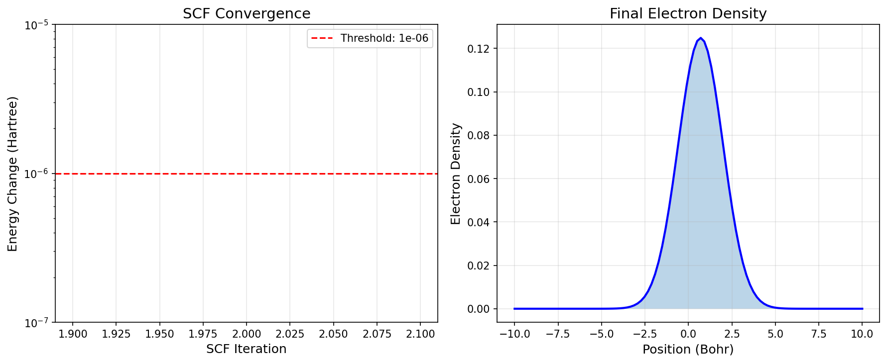
Terminal Output:

Computing H2 ground state energy...
--------------------------------------------------

SCF Convergence:
  Converged: True
  Iterations: 2

Energy Components (Hartree):
  Total Energy:             -2.899072
  Electronic Energy:        -3.614177
  Nuclear Repulsion Energy: 0.715104
  XC Energy:                -0.053951

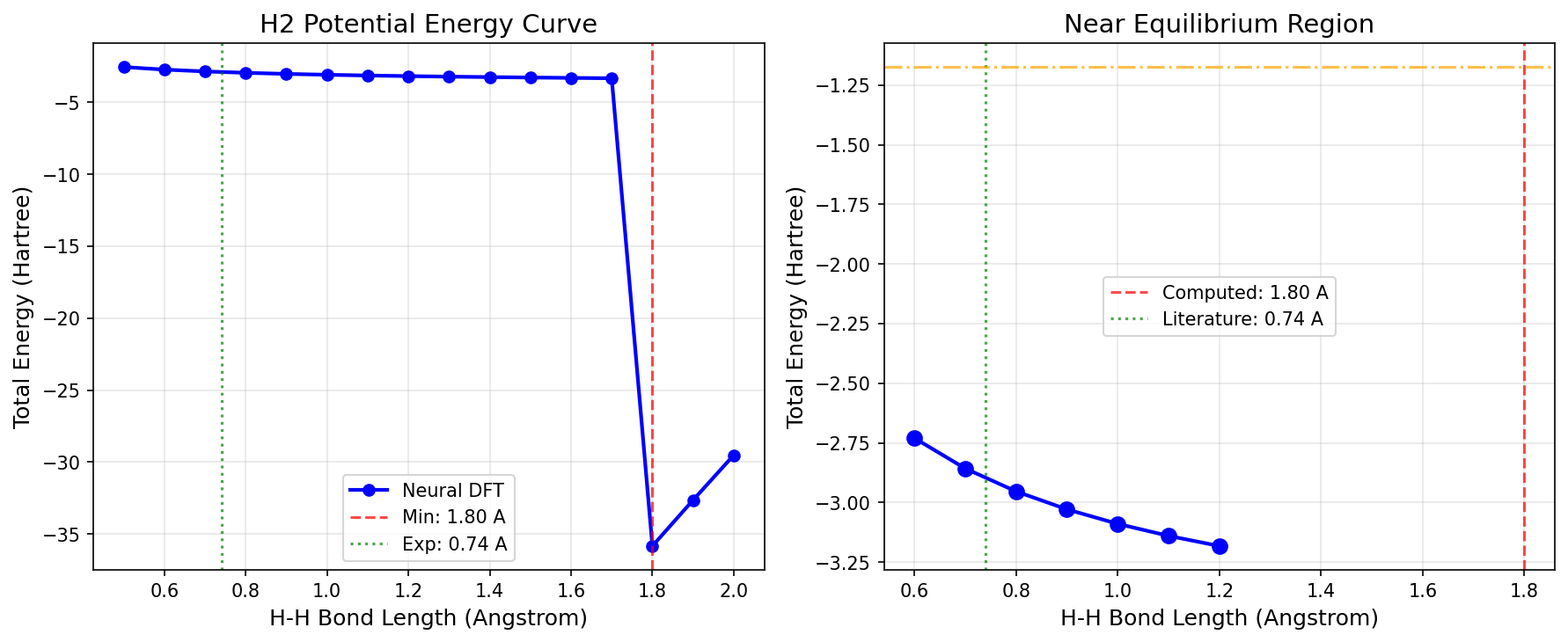
Step 4: Potential Energy Curve

bond_lengths = jnp.linspace(0.5, 2.0, 16)
energies = []

for bond_length in bond_lengths:
    h2 = create_molecular_system(
        atoms=[
            ("H", (0.0, 0.0, -float(bond_length) / 2)),
            ("H", (0.0, 0.0, float(bond_length) / 2)),
        ],
        charge=0, multiplicity=1,
    )
    result = neural_dft.compute_energy(h2, deterministic=True)
    energies.append(result.total_energy)

Terminal Output:

Computing Potential Energy Curve...
--------------------------------------------------
  Computed 4/16 points...
  Computed 8/16 points...
  Computed 12/16 points...
  Computed 16/16 points...

  PEC computation complete!
  Converged points: 16/16

  Equilibrium bond length: 1.800 Angstrom
  Equilibrium energy:      -35.828712 Ha

Visualization

Results Summary

Metric	Value
Molecular formula	H2
Number of electrons	2
Grid size	100
SCF converged	True
SCF iterations	2
Total Energy	-2.899 Ha
Reference Energy	-1.174 Ha
Training time	N/A (untrained)

Note: The neural DFT model is randomly initialized in this example and not trained on reference data. For production use, train the neural XC functional on high-level ab initio data (see the Neural XC Functional example).

Next Steps

Experiments to Try

1. Train the XC functional: Use the Neural XC training example to learn from LDA/GGA data
2. Different molecules: Try H2O, CH4 using create_water_molecule(), create_methane_molecule()
3. Higher precision: Increase grid_size for better accuracy
4. Compare methods: Use xc_functional_type="lda" for classical comparison

Related Examples

Example	Level	What You'll Learn
Neural XC Functional	Advanced	Train neural XC from reference data
First PINN	Beginner	Physics-informed approach
FNO on Darcy	Beginner	Data-driven operator learning

API Reference

• NeuralDFT: Main neural DFT framework class
• NeuralXCFunctional: Neural exchange-correlation functional
• NeuralSCFSolver: Neural-enhanced SCF solver
• MolecularSystem: Molecular system representation
• create_molecular_system(): Helper to create molecules from atoms
• DFTResult: Result dataclass with energy components

Troubleshooting

Issue	Solution
Poor energy accuracy	Train the neural XC functional on reference data
SCF not converging	Increase max_scf_iterations, reduce threshold
Memory issues	Reduce grid_size
Chemical accuracy not met	Use larger grid, train on more data

Current Limitations

The Neural DFT framework in Opifex is a research framework for developing new DFT methods. Current limitations include:

• 1D grid-based: Simplified grid representation vs. full 3D basis sets
• Untrained model: Neural components need training on reference data
• Research quality: Not production-ready for accurate energy calculations

For production quantum chemistry, consider using Opifex's neural XC functional with traditional DFT packages, or train on reference data from PySCF/Psi4.